Journal of Electromagnetic Analysis and Applications
Vol. 3 No. 5 (2011) , Article ID: 5025 , 6 pages DOI:10.4236/jemaa.2011.35028
Symbolic Computation and Graphic Presentation of Magneto-Static Field and Its Associated Vector Potential for a Steady Looping Current
![]()
University College, The Pennsylvania State University, York, USA.
Email: has2@psu.edu
Received January 4th, 2011; revised April 22nd, 2011; accepted April 27th, 2011.
Keywords: Magneto-Static Field of a Looping Current, Vector Potential, Symbolic Computation, Mathematica
ABSTRACT
With the advent of Computer Algebra System (CAS) such as Mathematica [1], challenging symbolic longhand calculations can effectively be performed free of error and at ease. Mathematica’s integrated features allow the investigator to combine the needed symbolic, numeric and graphic modules all in one interactive environment. This assists the author to focus on interpreting the output rather than exerting the efforts of relating the scattered separate modules. In this note the author, utilizing these three features, explores the magneto-static field and its associated vector potential of a steady looping current. In particular by deploying the numeric features of Mathematica the exact value of the vector potential of the looping current conducive to its 3D graph is presented.
1. Introduction and Motivation
In the course of quantifying the flux of a magnetodynamic field of a permanent mobile magnet through a certain planar conducting loop, the author needed to evaluate its companion static magnetic field. The evaluation of the latter entails modeling the current distribution within the permanent magnet. One such model deals with a current confined to the rim of a nut-shaped magnet. Other models extensively have been considered as well; for a comprehensive detailed analysis see Sarafian [2]. In the course of developing these models the author stumbled across a few issues of interest; surprisingly, none were addressed in the scientific literature. The lack of information was traced to pre-CAS era. Therefore, the thrust of this note is to provide the detailed procedure based on the application of a CAS such as Mathematica evaluating the magneto-static related quantities.
This note is composed of three sections. In addition to Introduction and Motivation, in Section 2, Analysis, we extend the current classic theoretical status of evaluating the vector potential and its associated magneto-static field of a steady looping current conducive to its 2D and 3D visual displays. In the last section we close the note with a few remarks.
2. Analysis
In general it is assumed that the electric current is the source of the magnetic field. The issue of interest is, “for a given current distribution, to evaluate its associated magnetic field.” Although in general one may apply Biot-Savart law [3] to evaluate the field, in practice one encounters mathematical challenges. Hence, in order to ease the mathematical difficulties one introduces a “simpler” mathematical object such as potential. Loosely speaking, the directional derivative of the potential yields the field. The theory of this methodology is classic and can be reviewed in detail almost in any upper level undergraduate as well as graduate physics textbooks, e.g. [4,5]. For a magneto-static field the potential is a vector; it is called vector potential, denoted by
 , and is related to the magnetic field,
 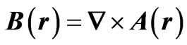 ,vector
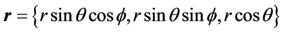
 represents the coordinates of an appropriately chosen coordinate system and
  is casted accordingly. Denoting the current density by
  the vector potential is given by [4,5],
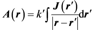 (1)
(1)
The integral is evaluated on the volume of the current distribution denoted with the volume element ; with
  being the observation point vector. The permeability of the free space in SI units is
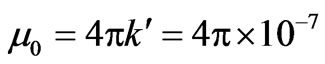 . We apply this formulation to a steady current i looping in a circle of radius a positioned on a horizontal plane centered about the origin of a coordinate system, see Figure 1.
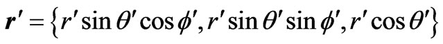
If one chooses a spherical coordinate system, the current density distribution ![]() can be written as,
can be written as,
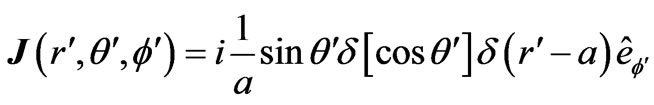 (2)
(2)
Here d is Dirac delta function, and  is the unit vector along the polar direction
  of the spherical coordinate system denoted with the vector
 . The denominator of (1) is
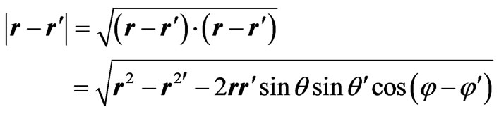
where we utilized
and
![]()
The volume element in (1) is
Upon substituting these pieces in (1) and integrating over  and
and  we arrive at
 . The f dependent of the potential is traced to
However, utilizing the symmetry of the current yields a f independent potential; that is to say irrespective the polar angle observation point the potential has the same value.
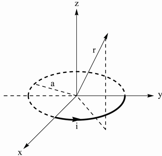
Figure 1. Display of a looping current i circulating a circular ring of radius a. The coordinate of the observation point is .
.
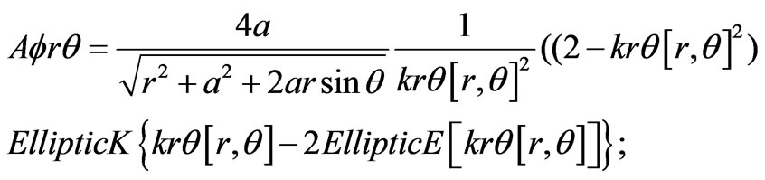
Setting f = 0 yields,
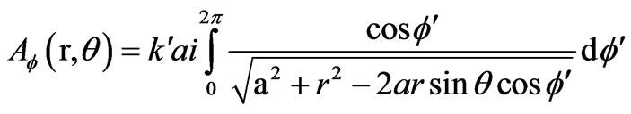 (3)
(3)
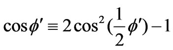
Equation (3) is evaluated analytically in [5]. Three steps are needed to deduce the output. First, replace  using the trigonometrical identity
In step 2, introduce a new variable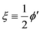 . By manipulating the integrand we get,
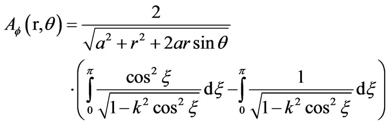 (4)
(4)
where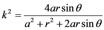 . In step 3, we recall the definition of the Complete Elliptical integral of the First and the Second kind, namely,
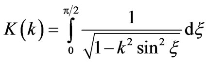
and
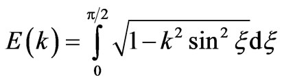
respectively. Then it is a matter of exercise to show these integrals are invariant after replacing  with
with . Hence, the second term of (4) yields 2 K(k). The integrand of the first term of (4) can be also manipulated as
 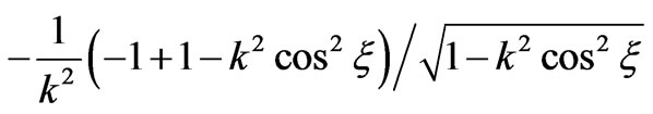 and the integration yields
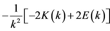 . Putting these pieces together we arrive at,
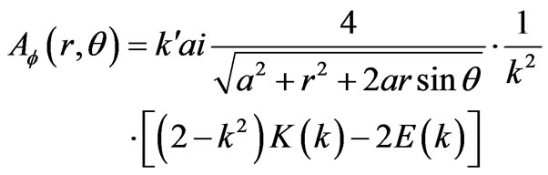 (5)
(5)
With this analytic expression at hand, we pursue evaluating its associated magnetic field. Applying the fundamental relationship between the vector potential and the field, namely,  , in a spherical coordinate system we write,
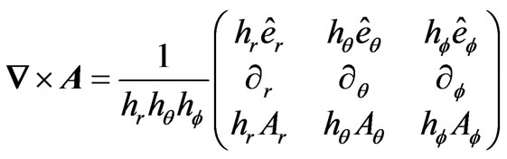 (6)
(6)
where the curvilinear scale factors are 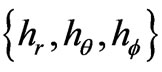
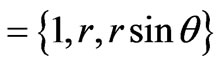 , [6]. Expanding the 3 × 3 determinant given in (6) yields the components of the magnetic field, namely,
 (7)
(7)
According to (5) the vector potential is an explicit function of elliptic integrals. Hence, it is not hard to envision that evaluating (7) is mathematically challenging. A thorough search reveals no such calculation has been reported in scientific literature. The classic textbook in electromagnetism, “Classical Electrodynamics”, Jackson [5] now in its third edition mnemonically refers to the components of the field, however does not explicitly provide the formulation. Without these explicit components it is hard to form an informed opinion about the magnetic field. One of the objectives of this note is to fill in the gap and complete the formulation of the problem at hand. Pursuing this goal in subsection Analysis a we utilize Mathematica and show how symbolically this is accomplished. In subsection Analysis b numerically we evaluate the vector potential and display its physical features. And in subsection Analysis c we display the 3D graph of the vector potential as well as the graphic relationship between the potential and the field.
2.1. Analysis a
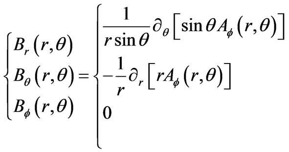
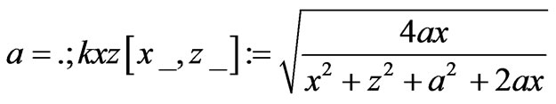
Utilizing (5 & 7) deploying Mathematica we symbolically evaluate the magnetic field. What follows are the needed Mathematica codes. In these codes EllipticK and EllipticE are the Mathematica library functions for the Complete Elliptic Integrals of the First and the Second kind, respectively.
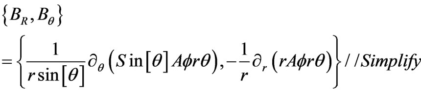
The radial and the azimuthal components of the magnetic field are denoted by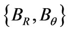 . These are:

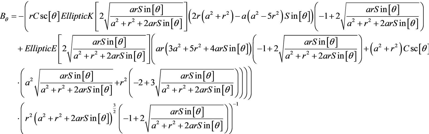
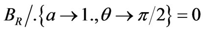
These expressions are the components of the magnetic filed at the position vector . For instance, for the given looping current, one intuitively expects that, on the horizontal plane, the radial component of the field to vanish. Since the azimuthal component of the field on the horizontal plane practically is along the vertical axis it should intuitively direct itself in two opposite vertical directions, depending on the point of interest being inside or outside of the loop. The latter observation conforms to the basis for one of the man made “Right Hand Rules”. For numeric evaluation and for simplicity we consider a loop with a one unit radius. Setting the azimuthal angle q = p/2 conforms to the horizontal plane. The next two code lines give the value of the radial component of the field and the plot of the azimuthal Bq (vertical Bz) field.
Plot[Evaluate[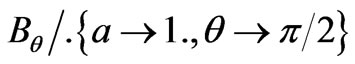 ], {r, 0.1, 2}, PlotStyle –> {Black,Thick}, AxesLabel –> {“r”, “~B = Bz”}, GridLines ® Automatic]
According to Figure 2, the field along the azimuthal (vertical) direction vanishes for the far points; an expected result. On the contrary for the points inside the ring they have the opposite sign i.e. they are directed in the opposite direction. While approaching the center of the ring the field behaves in the direction it is displayed.
2.2. Analysis b
Graphic display of the potential is missing in the scientific literature; this hinders ones physical insight. Utilizing Mathematica graphics, we fill in the gap. To accomplish this, it is helpful to plot the contours of the potential about the ring. Utilizing the symmetry of the ring we plot the contours only on the xz-plane. First we change the coordinate system from spherical to its associated Cartesian coordinate. This requires replacing x = rsinq. This
Figure 2. Display of the azimuthal Bq (vertical Bz) component of the magnetic field on the horizontal plane of a current, looping in a circular loop of radius one unit. The asymptote of the field occurs at r = a = 1. The field changes sign/direction around the rim of the loop.
also entails reformatting the argument of the elliptical integrals. The code reads,
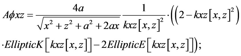
contourplotExactzoomed = ContourPlot[Afxz/.a®1, {x, 0, 2}, {z, –1, 1}, ContourShading ® False, ContourStyle ® Thick, GridLines ® Automatic, FrameLabel ® {“x”, “z”}]
disk=Graphics[Disk[{1,0},0.02]];
Show[{contourplotExactzoomed,disk}]
This graph assists in forming an opinion about the polar component of the magnetic vector potential. In other words, it shows for the points close to the rim of the ring the potential contours are closed loops asymmetrically wrapped around the ring. For the points near by the symmetry axis, the contours are open; they are almost straight lines parallel to the symmetry axis. For the outside far points the contours are open curves; the further the points are from symmetry axis the curves are less bent.
Figure 3 also shows that there is a transition interior region where the closed contours break away forming open curves. Zooming in this feature we make a series of plots animating the contour transitions.
tableContourN = Table[Show[{ContourPlot[Evaluate [Afxz/.a ® 1] == n, {x, 0, 2}, {z, –1, 1}, ContourShading ® False, ContourStyle ® Thick, GridLines ® Automatic, Frame Label ® {“x”, “z”}](*{n, 2.9, 3.1, 0.1}*), disk}], {n, 3.15, 2.9, –0.05}]
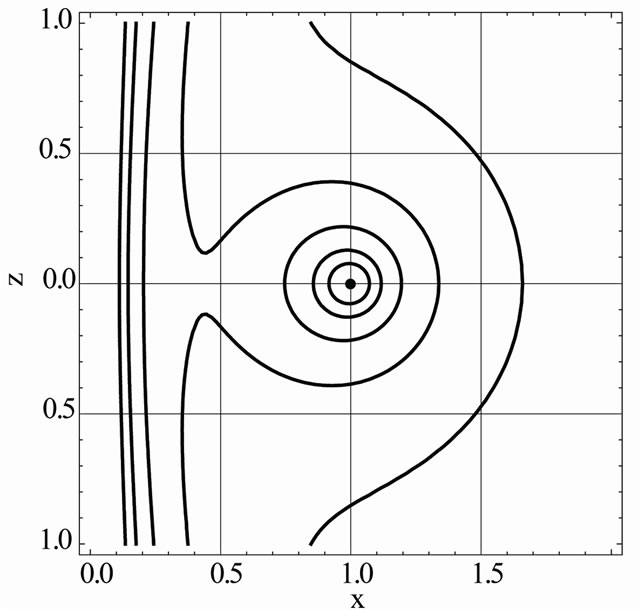
Figure 3. The contour plots of the vector potential Af(x,z) on the xz-plane. The dot at the center of the graph is the cross section of the current carrying loop.
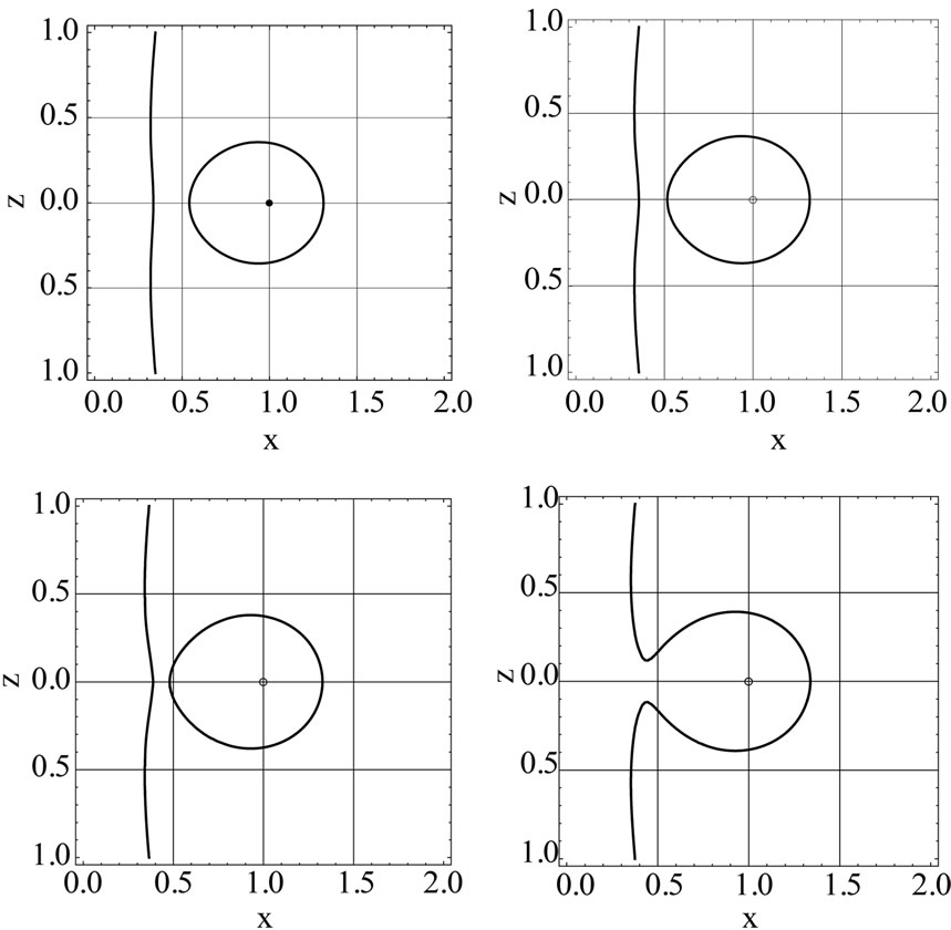
Figure 4. Frames of the contour plots of the vector potential  on the xz-plane. The frames show the shape shifting mutation from the break away configuration to the joined contour phase.
In other words, plots shown in Figure 4 are a series of individual refined collective contours of Figure 3. Exe-cuting the Mathematica code given at the top of the Figure 4 animates the plots bringing the transition of the plotted graphs to life.
2.3. Analysis c
Applying 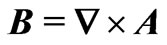 we may now visualize the magnetic field. The fields are tangent to the potential curves, i.e. the contours and the fields are on the same plane. The fields are plotted applying Mathematica StreamPlot. In doing so first we replace the spherical coordinate system with its associated Cartesian coordinate. We then zoom in three different areas: the entire region, the region close to the center and the region far from the loop. These are shown sequentially in Figure 5.
These plots show the relationship between the potential and the field. For instance the first graph shows how the field in order to sustain its tangential alignment reorients itself; compare this feature vs. the field for the points close to the rim and the ones close the center. One readily may observe useful features analyzing the second and the third graphs as well.
We further our analysis by displaying three 3D graphs for the vector potential Figure 6; these are also missing in literature. These surfaces are formed by revolving a hand full of potential contours displayed in Figure 3 about the symmetry axis in the spherical coordinate system.
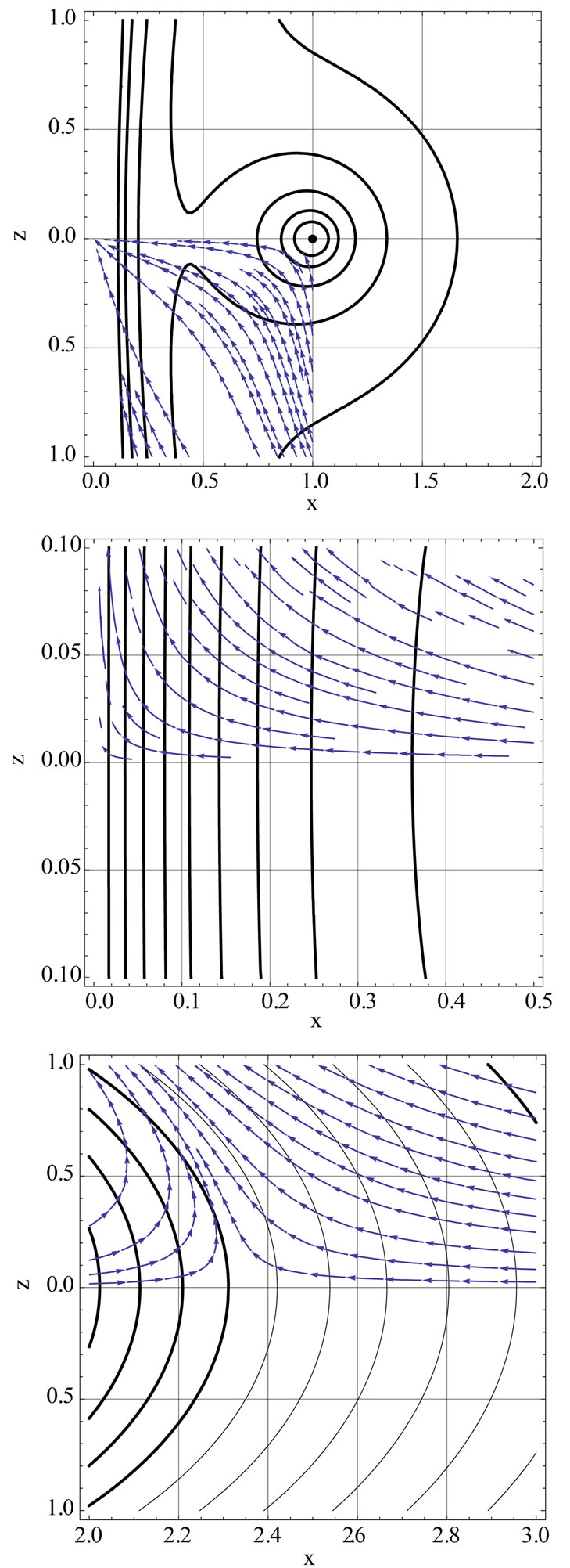
Figure 5. The black curves are the vector potential on the xz-plane. The field lines are shown with vectors.
tableSpherical3DN = Table[SphericalPlot3D[Afrq/.a ® 1.,{q, 0, p}, {f, 0, p}, Mesh ® False, PlotStyle ® Directive[Hue[0.2r], Opacity[0.7], Specularity[White, 10], ImageSize®600,PlotRange ® {{–1, 1}, {–1, 1}, {–5, 5}}]], {r, 0.01, 3, 0.5}]
Figure 6. 3D plots of the vector potential resulting from revolving the 2D contour plots of the potential about the symmetry axis of the ring.
In many words, the magnetic vector potential is a 3D function. For the best scenario its 2D profile utilizing Mathematica contour plot is depicted in Figures 3 and 4. Here in Figure 6 we have displayed its 3D actual being conducive to a better understanding of the problem at hand. This is missing in scientific literature.
In Figure 6 from left to right the plots corresponding to the contour potentials associated with the radial distance r = 0.01 to 1.01 at 0.5 step increments. As expected these surfaces are symmetric about the axis of the ring. The bulging area of the surfaces is associated with the curvature of the associated 2D contours.
3. Conclusions
Traditional methodology of mathematical physics with the advent of Computer Algebra System (CAS) has gone through a quantum transition. CAS can assist and minimize the tedious longhand symbolic calculations requiring time consuming efforts that once hindered the exploration of new horizons. Numeric computation of issues of interest as well as their accompanied graphs utilizing CAS is a norm of mathematical physics. Consequently, the authors of scientific academic textbooks are encouraged to utilize CAS to present results. An example of how these features are culminated conducive to a comprehensive research project is presented in this note. The author systematically following the traditional steps of mathematical physics has tackled a topic of interest utilizing a CAS such as Mathematica bringing the project to fruition. The details discussed in this project are an example demonstrating how Mathematica plays an essential role exploring new features not yet reported in scientific literature. The entire project including the text is completed utilizing the latest version of Mathematica, V 8.0.1 [7]. A thorough literature search has been completed by the author; since this project is a novel concept without previous studies, he is unable to augment the reference list beyond its current status.
4. Acknowledgement
The author would like to thank Mrs. Nenette Sarafian Hickey for carefully reading over the manuscript and making editorial comments.
REFERENCES
- S. Wolfram, “The Mathematica Book,” 4th Edition, Cambridge, 1999.
- H. Sarafian, “A Halo Current and the Magnetic Field of a Nut-Shaped Magnet, Invited Paper, Research Institute for Mathematical Science (REMS),” Kyoto University, Japan, in Press, 2011.
- D. Halliday, R. Resnik and J. Walker, “Fundamental of Physics,” 9th Edition, Wiley and Sons, Hoboken, 2010.
- J. Reitz and F. Milford, “Foundations of Electromagnetic Theory,” Addison-Wesley Publishing Company Inc., Boston, 1960.
- J. D. Jackson, “Classical Electrodynamics,” 3rd Edition, John Wiley, Hoboken, 1998.
- M. Spiegel, “Vector Analysis,” Schaum Series, 1959.
- Mathematica V 8.0.1, Wolfram Research Inc., Champaign, 2011.