Journal of Electromagnetic Analysis and Applications
Vol. 3 No. 6 (2011) , Article ID: 5353 , 6 pages DOI:10.4236/jemaa.2011.36035
On Chebyshev Array Design Using Particle Swarm Optimization
![]()
Department of Electrical Engineering, Faculty of Engineering, Qassim University, Qassim, Saudi Arabia.
Email: mohbat@qec.edu.sa
Received March 10th, 2011; revised March 20th, 2011; accepted April 12th, 2011.
Keywords: Optimization, PSO, Linear Antenna Arrays, Chebyshev Radiation Pattern
ABSTRACT
In this paper, the evolutionary algorithm of particle swarm optimization (PSO) is applied to synthesis an optimal linear array in the Chebychev sense. Equiripple radiation patterns may be obtained by synthesizing the excitation currents feeding the array or by carefully choosing the interelement spacing. The desired equal side lobes level is achieved simultaneously with the narrowest possible beamwidth (high directivity). Though the optimization problem may become nonlinear, convex and/or sometimes nonconvex, it can be handled using an efficient, a robust and a nongradient based particle swarm optimizer algorithm. In order to effectively utilize this algorithm it is important to define an appropriate objective, or cost, function that return a single number to enable the PSO algorithm minimizing it. In this paper, the objective function is formulated taking into consideration the level of the side lobes as well as the main beam width. In addition to satisfy the objective function, the obtained results using the proposed technique are in agreement with those available in the literature.
1. Introduction
When antennas elements are arrayed in a certain geometrical configuration the signal induced on them are combined to form the array output. A plot of the array response as a function of angle is normally referred to as the array pattern or beam pattern. Synthesizing the array pattern of antenna arrays has been a subject to several studies and investigations. The trade-off between the side-lobe levels (SLL) and the half-power beamwidth (HPBW) stimulate the question answered primarily by Dolph [1] of obtaining the narrowest possible beamwidth for a given side-lobe level or the smallest side-lobe level for a given beamwidth. This was possible by using the orthogonal functions of Chebyshev [2] in order to design an optimum radiation pattern. However, for large number of elements this procedure becomes quite cumbersome since it requires matching the array factor expression with an appropriate Chebyshev function [3]. To overcome this deficiency, Safaai-Jazi [4] proposed a new formulation for the design of Chebyshev arrays based on solving a system of linear equations. Iterative procedure was used to produce the desired pattern [5]. Formulating the synthesis problem as a convex optimization, which may be solved by interior-point methods, has been presented in [6]. Shpak et al. [7,8] discussed an improved method for the design of linear arrays with prescribed nulls. The forgoing mentioned investigations either require analytical formulae or evaluating the gradient of some cost function, which sometimes become formidable to evaluate. As alternatives, neural network and evolutionary algorithms techniques were used in order to reduce the side lobes of linear arrays [9,10]. Genetic algorithms (GA) and particle swarm optimization are well-known evolutionary algorithm techniques. In GA, a sample of possible solutions is assumed then mutation, crossover, and selection are employed based on the concept of survival of the fittest [10]. On the other hand, PSO is a much easier algorithm in which each possible solution is represented as a particle in the swarm with a certain position and velocity vector [11,12]. The position and velocity of each particle are updated according to some fitness function [11]. Some studies have been devoted to compare between the GA and PSO [20,21] and a general conclusion has been reached the PSO shows better performance due to its greater implementation simplicity and minor computational time.
Since it has been introduced by Kennedy and Eberhard [13], the PSO is being applied to many fields of endeavor. Surprisingly, it has been applied to the design of low dispersion fiber Bragg gratings [14], and to the design of corrugated horn antenna [15]. Other applications can be found in [16]. This investigation is devoted to the design of Chebyshev linear antenna arrays by considering various affecting parameters using the PSO. The paper is organized as follows. In Section II, the particle swarm optimization algorithm is overviewed. A background about Chebyshev polynomials is addressed in Section III. Formulation of linear array pattern synthesis is presented in Section IV. Simulation examples and results are given in Section V. Conclusions drawn and hints to further investigation are pointed out in Section VI.
2. Particle Swarm Optimization (PSO) Algorithm
PSO is a stochastic optimization technique that has been effectively used to solve multidimensional discontinuous optimization problems in a variety of fields [17]. The stochastic behavior of this technique can be controlled by one single factor which can be chosen to end up with a deterministic strategy that does not need gradient information. Compared with other evolutionary 9 techniques, the PSO is much simpler and easier to implement with guaranteed convergence [18].
The concept of the PSO is derived from an analogy of the social behavior of a swarm of bees in the field, for example. Without any prior knowledge, each bee referred to as agent or particle in the PSO jargon, in the swarm starts with random position and velocity with an aim to find the location of highest density of flowers in the field. Then, during their search, each bee updates its velocity and position based on two pieces of information. The first is its ability to remember the location of most flowers it personally found (particle best will be denoted later as pbest). The second represents the location of most flowers found by all the bees of the swarm (global best will be denoted later as gbest) at the present instant of time. This process of updating velocities and positions continues and will result in one of the bees would find a location with a highest density of flowers in the field. Eventually, all the bees (solutions) will be drawn to this location since they will not be able to find any other better location. This represent a convergence of the algorithm and the optimum solution is obtained [11,13,17, 20-24]. The main steps of the PSO algorithm are given below and will be elaborated in the remaining portion of this section.
1) Definition of the solution space: In this step, the minimum and maximum value for each dimension in the N-dimensional optimization problem are specified to define the solution space of the problem.
2) Definition of the fitness function: The fitness function is a problem dependent measure of the goodness of a position (N-dimensional vector) that represents a valid solution of the problem. It should be carefully selected to represent the goodness of the solution and return a single number.
3) Random initialization of the swarm positions and velocities: The positions and velocities of the particles are randomly initialized. To help the discussion let us refer to these matrices as X and V, respectively. Both matrices have a dimension of M ´ N. Here, M represents the number of particles or swarm size and N represents the dimension of the optimization problem. However, it is preferred to randomly initialize the X matrix within the solution space for faster convergence. To complete the initialization step, each row in the matrix X is labeled as the individual best position for each particle (pbest). In addition, the positions in X are plugged into the fitness function and the returning numbers are compared, the position with the best returning number is labeled as the global best position (gbest). In this context, the word best could mean highest or lowest depending on the optimization problem. The problem considered here is a minimization of the fitness function.
4) Update of velocity and position: The following sub-steps are carried out for each particle individually:
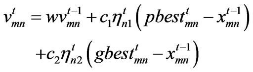
a) Velocity update: The velocity of the mth particle in the nth dimension is updated according to the following equation
 (1)
(1)
The superscripts t and t–1 denote the time index of the current and the previous iterations, hn1 and hn2 are two different, uniformly distributed random numbers in the interval [0,1]. The relative weights of the personal best position versus the global best position are specified by the parameters c1 and c2, respectively. Both c1 and c2 are typically set to a value of 2.0 [19]. The parameter w is called the “inertial weight”, and it is a number in the range [0,1] that specifies the weight by which the particle’s current velocity depends on its previous velocity, and the distance between the particle’s position and its personal best and global best positions. Empirical studies [11] have shown that the PSO algorithm converges faster if w is linearly damped with iterations, for example starting at 0.9 at the first iteration and finishing at 0.4 in the last iteration.
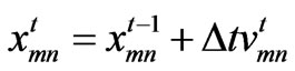
b) Position update: In this step, the position of the mth particle in the nth dimension is updated according to the following equation
 (2)
(2)
where  represents a given time step (usually chosen to be one).
c) Fitness evaluation: The updated N-dimension position in the previous step is plugged in the fitness function and the returning number is compared with that corresponding to the pbest, if the returning number is better, this updated N-dimension position is labeled as the new pbest. In addition, if the returning number is better than that corresponding to gbest, the updated N-dimension position is also labeled as the new gbest.
5) Checking the termination criterion: In this step, the algorithm may be terminated if the number of iteration equals a pre-specified maximum number of iteration or the returning number corresponding to gbest is close enough to a desired number. If none of the above conditions is satisfied, the process is repeated starting at step 4.
3. Chebyshev Polynomials
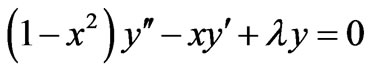
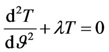
One of the most eminent methods used to equate the sidelobes arising in the radiation pattern of antenna arrays is to utilize a set of polynomials referred to as Chebyshev polynomials, after the Russian mathematician Pafnuti Chebyshev (1821-1894) [2]. These polynomials are originated as possible solutions of a second order ordinary differential equation with variable coefficients. This eigenvalue equation may take the form
 (3)
(3)
with an additional requirements that y(–1),  (–1), y(1), and
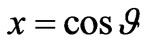
  (1) are to be bounded. A change of variables according to
 (4)
(4)
transforms Equation (3) to
 (5)
(5)
where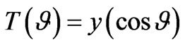 . The transformation used in Equation (4) results in a second order linear ordinary differential equation with constant coefficients as given by Equation (5). Solutions of Equation (5) depend on the eigenvalue l and could be written as
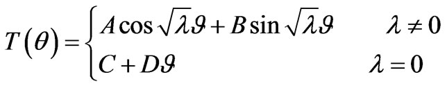 (6)
(6)
where A, B, C, and D are arbitrary constants. The solution would be bounded if B = D = 0 and 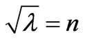 with n being an integer. The eigenfunctions, corresponding to nontrivial solutions are given by
 (7)
(7)
In terms of the original independent variable x, the eigenvalues and eigenfunctions are given by
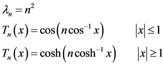 (8)
(8)
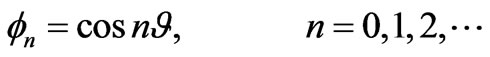
Here, the dependent variable T is in honor of Chebyshev (often spelled Tchebysceff). Using the Euler identity and substituting for x from Equation (4), the argument  could be expanded in terms of its fundamental argument,
 . A few examples are given below, for different orders, for the purpose of illustration
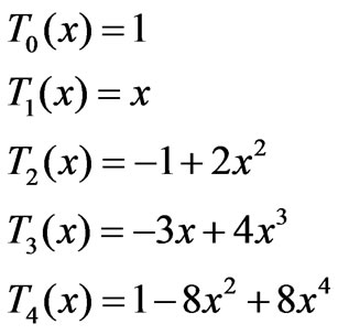 (9)
(9)
A general recursion formula may be deduced from Equations (9) and is given by
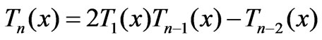 (10)
(10)
Chebyshev polynomials constitute a set of orthogonal functions with respect to a weighting function, . The weighting function could be found be recasting Equation (7) in standard Sturm-Liouville form. Carrying out this step to find [2]
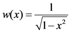 (11)
(11)
With respect to this weighting function, Chebyshev polynomials are orthogonal, i.e., they satisfy
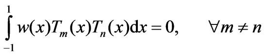 (12)
(12)
These polynomials oscillate with unit amplitude in the interval  and become monotonically increasing or decreasing, depending on their order, outside this range. This property of Chebyshev polynomials enabled Dolph to use them to design an equiripple radiation patterns.
4. Linear Array Pattern Synthesis
The focus here will be on an N-element array distributed on a line with equal interelement spacing, d. The array factor may be written as
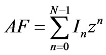 (13)
(13)
Here,  and
and . The angle q is measured from the line of the array, the wavenumber k = 2p/l; l being the wavelength, and b is the difference in phase excitation between the elements. In is the magnitude of the current of the nth element. For symmetrical current distribution Equation (13) may be written as [3]
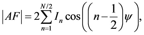 (14)
(14)
for even number of elements. In the case of odd number of elements, the array factor could be written as [3]
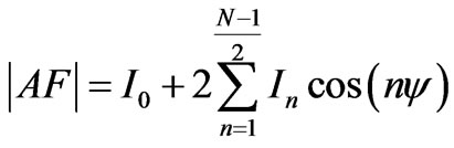 (15)
(15)
In Equation (15), I0 denotes the current of the center element. The case of unequal interelement spacing will be considered also. This requires a straightforward modification in Equations (14) and (15), however. The correspondence between an N-element array factor (Equation (14) and Equation (15)) and a Chebyshev polynomial of order (N – 1) is carried out to match the coefficients of similar terms thus giving the required current excitations . It is clear that this procedure requires elaborate computation especially for large number of elements. The problem is circumvented here as an optimization one. Starting from an arbitrary, or random, current excitation, the PSO algorithm is used in order to return current excitation that leads to an equiripple pattern with the narrowest possible beamwidth. The procedure of using the PSO to obtain the required current excitations
  may be summarized in the following steps 1) Specify N, d, and b.
2) Start with an arbitrary current excitation .
.
3) Obtain the array factor AF ( ) using either Equation (14) or (15).
4) The side-lobe levels  and their locations
  are determined to be used in the next step;
 . Here,
  denotes the number of peaks appear in side-lobe regions.
5) The side-lobe levels  are forced not to exceed a certain level, say c, and this is achieved by minimizing the following cost, or fitness, or error, or objective function
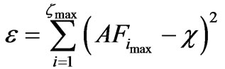 (16)
(16)
6) Return to step 2 while the number of iterations or minimum error criteria is not attained, otherwise stop. Indeed the process described above gave equiripple radiation pattern but not necessarily the narrowest possible beamwidth. Thus the cost function should be amended to incorporate a condition on the beamwidth also. Equation (16) is therefore modified to read
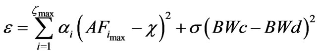 (17)
(17)
The positive weighting factors ai and s are added to give each factor a certain influence on the obtained results. The numerically calculated beamwidth (BWc) is compared with the desired beamwidth (BWd), which may be determined by an analytic formula (e.g. [4]). Equation (17) satisfies the requirement of the PSO algorithm that the fitness function should return a single number representing the target of the minimization process. The optimization here is carried out using a fixed spacing, which is l/2, between the elements. However, this spacing is not an optimum spacing. Looking for such an optimum spacing is also undertaken. Using an optimum spacing, which is usually greater than l/2, extends the visible space. Hence, more sidelobes and narrower patterns are expected. To further demonstrate the capabilities of the PSO algorithm, the locations of the array elements are also considered as the optimized parameters. Though the problem becomes nonlinear, the PSO returned the required spacings that lead to equiriple pattern. These points will be elaborated by considering specific examples in the following Section.
5. Illustrative Examples
In this section, the capabilities of the PSO algorithm in the synthesis of antennas array are demonstrated by three examples. First, the PSO algorithm was used to find the current excitations that result in equiripple array factor. In this example, the interelement spacing was set to l/2 and all excitation currents are assumed to be equiphase. Figure 1 shows the radiation pattern of a 10-element array using the excitation currents returned by the PSO with fitness function as defined in Equation (16) (dotted line) and in Equation (17) (solid line). In the former case, the goal was to obtain an equiripple array with side lobes level of –20 dB. Although the side lobes are at the desired level, the obtained array is not optimum in a Chebyshev sense. To overcome this problem, the fitness function was modified as given in Equation (17) to achieve the narrowest possible main lobe besides obtaining an equiripple pattern. With this modification of the fitness function, the PSO returned excitation currents that resulted in the desired narrow main lobe and equal side lobe level. The returned current excitations of this case along with various other examples using different array sizes are given in Table 1. These results are in excellent agreement with those presented elsewhere (e.g. [4]). In the second example, the PSO was used to find more directive patterns than that obtained by limiting the spacing between the elements to l/2. Such optimum spacing undoubtedly extends the visible space and results
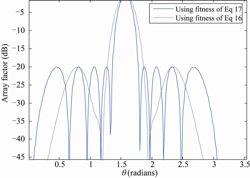
Figure 1. Radiation pattern of 10-element antennas array synthesized using PSO using two different fitness functions.
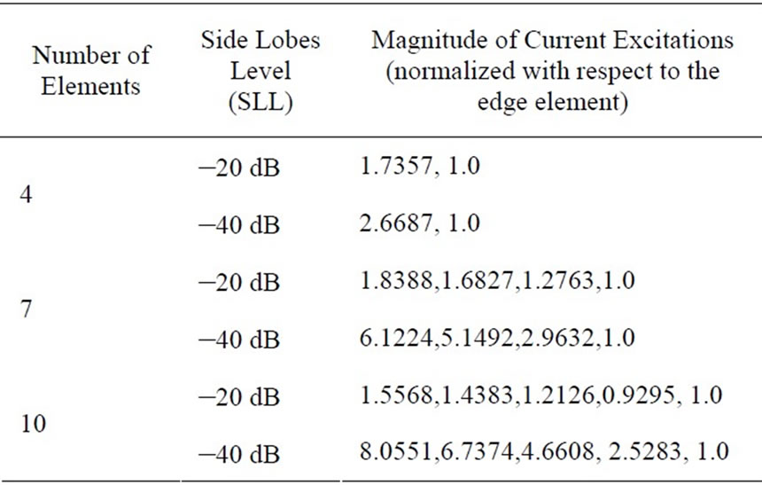
Table 1. Magnitude of Current Excitation of l/2-spacing for antenna array synthesis using PSO.
in more side lobes accommodated in the radiation pattern.
For a 10-element array with 20 dB SLL the optimum spacing returned by the PSO algorithm is 0.8964 l. This is in excellent agreement with the result obtained using the analytic expression given in [4]. Figure 2 shows the radiation patterns obtained by using this spacing and that by using half wave spacing.
The convergence of the algorithm toward this value is shown in Figure 3 for agent number 15 for iterations from 110 to 170. As the figure indicates, beyond the 140th iteration the value settled to the optimum value.
In the third example, the PSO was used to find the locations of the array elements to achieve a desired equal side lobe level and the narrowest possible beam width. The current excitation is assumed to be uniform in this case. Figure 4 shows the radiation pattern of a 10-element antenna array achieved by changing interelement spacings in order to get 20 dB side lobe level. For comparison, the radiation pattern of the same array with half wave spacing which has side lobe at higher levels is shown in the figure.
As Figure 4 shows, the desired side lobe level is achieved. The interelement spacing (returned by the PSO) for this case and some other cases are given in Table 2.
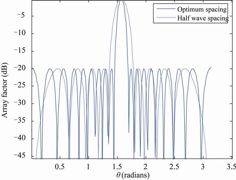
Figure 2. Radiation pattern of 10-element antennas array with optimum and half wave spacing.
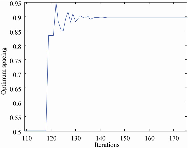
Figure 3. Convergence of the optimum spacing versus number of iterations.
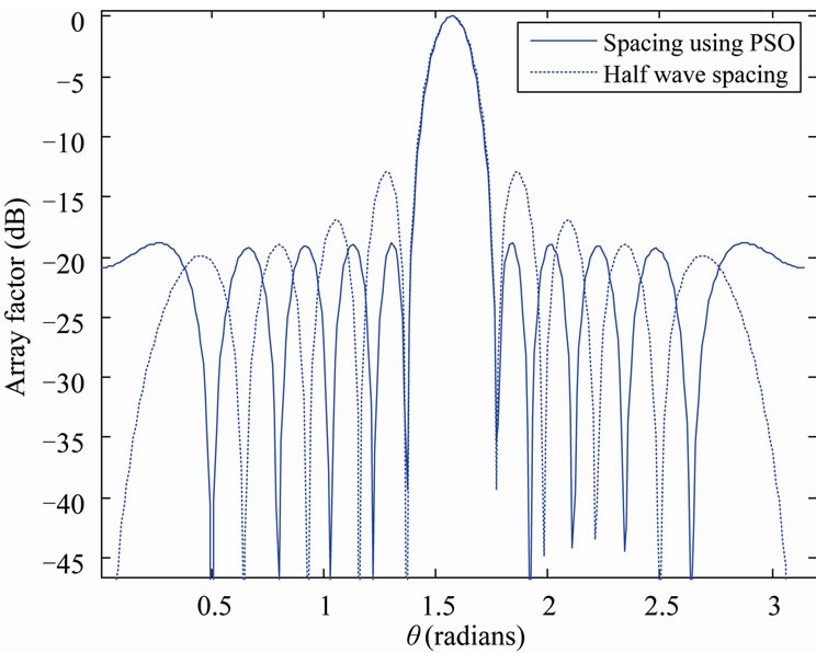
Figure 4. Radiation pattern of 10-element antenna with locations obtained using PSO and half wave spacing uniform array.
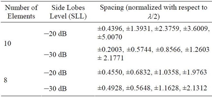
Table 2. Unequal Spacings for antenna array (with uniform current excitation) Synthesized Using PSO.
The spacings in Table 2 are the distance between the center of the array and the corresponding element.
6. Conclusions
The application of PSO to design chebyshev arrays has been demonstrated in this paper. The objective function has been carefully defined in order to obtain accurate results. Current excitations and the locations of the array elements are optimized to obtain the anticipated aim. General nonuniform arrays have been designed and the results are in agreement with those reported in the literature. The proposed method of PSO can also be utilized to place a controlled null anywhere in antenna pattern and this would be useful in suppressing unwanted interferences.
REFERENCES
- C. Dolph, “A Current Distribution for Broadside Arrays which Optimizes the Relationship between Beamwidth and Side Lobe Level,” Proceeding IRE, Vol. 34, No. 5, 1946, pp. 335-348.
- M. Greenberg, “Advanced Engineering Mathematics,” Prentice-Hall, Upper Saddle River, 1998.
- Balanis, “Antenna Theory Analysis and Design,” 3rd Edition, John Wiley, New York, 2005.
- A. Safaai-Jazi, “A New Formulation for the Design of Chebyshev Arrays,” IEEE Transactions on Antennas and Propagation, Vol. 42, No. 3, 1994, pp. 439-443.
- S. Nagesh and T. Vedavathy, “A Procedure for Synthesizing a Specified Sidelobe Topography Using an Arbitrary Array”, IEEE Transactions on Antennas and Propagation, Vol. 43, No. 7, 1995, pp. 742-745.
- H. Lebret and S. Boyd, “Antenna Array Pattern Synthesis via Convex Optimization,” IEEE Transactions on Signal Processing, Vol. 45, No. 3, pp. 526-532. 1997. doi:10.1109/78.558465
- D. Shpak and A. Antoniou, “A Flexible Optimization Method for the Pattern Synthesis of Equispaced Linear Arrays with Equiphase Excitation,” IEEE Transactions on Antennas and Propagation, Vol. 40, No. 10, 1992, pp. 1113-1120.
- D. Shpak, “A Method for the Optimal Pattern Synthesis of Linear Arrays with Prescribed Nulls,” IEEE Transactions on Antennas and Propagation, Vol. 44, No. 3, 1996, pp. 286-294,
- M. Dahab, K. Hijjah and S. Khamy, “A New Technique for Linear Array Processing for Reduced Sidelobes Using Neural Networks,” Proceedings of the Fifteenth National, Cairo, 24-26 Feb 1998.
- Y. Rahmat-Samii and E. Michielssen, “Electromagnetic Optimization by Genetic Algorithms,” Wiley, New York, 1999.
- J. Robinson and Y. Rahmat-Samii, “Particle Swarm Optimization in Electromagnetics,” IEEE Transactions on Antennas and Propagation, Vol. 52, No. 2, 2004, pp. 397-402.
- D. Boeringer and D. Werner, “Particle Swarm Optimization versus Genetic Algorithms for Phased Array Synthesis,” IEEE Transactions on Antennas and Propagation, Vol. 52, No. 3, 2004, pp. 771-779.
- J. Kennedy and R. Eberhart, “Particle Swarm Optimization,” Proceeding of IEEE Conference of Neural Network IV, Piscataway, 1995.
- S. Baskar, R. Zheng, A. Alphones, N. Ngo and P. Suganthan, “Particle Swarm Optimization for the Design of Low Dispersion Fiber Bragg Gratings,” IEEE Photonics Technology Letters, Vol. 17, No. 3, 2005, pp.615-617. doi:10.1109/LPT.2004.840924
- J. Robinson, S. Sinton and Y. Rahmat-Samii, “Particle Swarm, Genetic Algorithm, and Their Hybrids: Optimization of a Profiled Corrugated Horn Antenna,” IEEE Antennas and Propagation Society International Symposium, Vol. 1, 2002, pp. 314-317.
- Y. Rahmat-Samii and C. Christodoulou, “Special Issue on Synthesis on Synthesis and Optimization Techniques in Electromagnetic and Antenna System Design,” IEEE Transactions on Antennas and Propagation, Vol. 55, No. 3, 2007, pp. 518-522. doi:10.1109/TAP.2007.891879
- R. C. Eberhart and Y. Shi, “Evolving Artificial Neural Networks,” Proceeding of International Conference of Neural Networks Brain, Beijing, 1998.
- J. Kennedy and W. M. Spears, “Matching Algorithm to Problems: An Experimental Test of the Particle Swarm and Genetic Algorithms on Multimodal Problem Generator,” Proceeding IEEE International Conference of Evolutionary Computation, 1998.
- I. C. Trelea, “The Particle Swarm Optimization Algorithm: Convergence Analysis and Parameter Selection,” Information Processing Letters, Vol. 85, No. 6, 2003, pp. 317-325. doi:10.1016/S0020-0190(02)00447-7
- D. W. Boeringer and D. H. Werner, “Particle Swarm Optimization versus Genetic Algorithms for Phased Array Synthesis,” IEEE Transactions on Antennas and Propagation, Vol. 52, No. 3, 2004, pp. 771-779. doi:10.1109/TAP.2004.825102
- R. Shavit and I. Taig, “Array Pattern Synthesis Using Neural Networks with Mutual Coupling Effect,” IEEE Proceeding of Microwave Antennas Propagation, Vol. 152, No. 5, 2005, pp. 354-358. doi:10.1049/ip-map:20045121
- K. Guney and N. Sarikaya, “A Hybrid Method Based Combining Artificial Neural Network and Fuzzy Inference System for Simultaneous Computation of Resonant Frequencies of Recetngular, Circular, and Triangular Microstrip Antennas,” IEEE Transactions Antennas and Propagation, Vol. 55, 2007, pp. 659-668. doi:10.1109/TAP.2007.891566
- S. Selleri, M. Mussetta, P. Pirinoli, R. E. Zinch and L. Matekovits, “Differentiated Meta-PSO Methods for Array Optimization,” IEEE Transactions on Antennas and Propagation, Vol. 56, No. 1, 2008, pp. 67-75.
- W. Li, W. Shi, Y. Hei, S. Liu and J. Zhu, “A Hybrid Optimization Algorithm and Its Application for Conformal Array Pattern Synthesis,” IEEE Transactions on Antennas and Propagation, Vol. 58, No. 10, 2010, pp. 3401-3406. doi:10.1109/TAP.2010.2050425