Journal of Intelligent Learning Systems and Applications
Vol. 5 No. 1 (2013) , Article ID: 28065 , 10 pages DOI:10.4236/jilsa.2013.51007
Genetic Optimization of Artificial Neural Networks to Forecast Virioplankton Abundance from Cytometric Data
![]()
Civil Engineering Program, Federal University of Rio de Janeiro, Center of Technology, Fundão Island, Rio de Janeiro, Brasil.
Email: *marilia@coc.ufrj.br
Received October 1st, 2012; revised December 17th, 2012; accepted December 24th, 2012
Keywords: Virioplankton Prediction; Flow Cytometry; Neural Networks; Genetic Algorithm; Trophic Gradients
ABSTRACT
Since viruses are able to influence the trophic status and community structure they should be accessed and accounted in ecosystem functioning and management models. So, this work met a set of biological, chemical and physical time series in order to explore the correlations with marine virioplankton community across different trophic gradients. The case studied is the Arraial do Cabo upwelling system, northeast of Rio de Janeiro State in Southeast coast of Brazil. The main goal is to evolve three type of artificial neural network (ANN) by genetic algorithm (GA) optimization to predict virioplankton abundance and dynamic. The input variables range from the abundance of phytoplankton, bacterioplankton and its ratios acquired by one in situ and another ex situ flow cytometers. These data were collected with weekly frequency from August 2006 to June 2007. Our results show viruses being highly correlated to their host, and that GA provided an efficient method of optimizing ANN architectures to predict the virioplankton abundance. The RBF-NN model presented the best performance to an accuracy of 97% for any period in the year. A discussion and ecological interpretations about the system behavior is also provided.
1. Introduction
Nowadays, viruses are considered ubiquitous, active and ecologically important members of microbial communities influencing biogeochemical cycles, community composition and horizontal gene transfer [1-3]. Many reports have described them along several environments [4-7]. The use of transmission electron microscopy (TEM) for aquatic virus investigation [8] was followed by the epifluorescence microscopy (EFM) along with the development of a variety of highly fluorescent nucleic acid dyes [9]. More recently, flow cytometry (FCM) emerged as a new method, because it is a faster technology for direct counts [10-12]. Since then, FCM has been applied successfully to analyze microbial communities [13-16]. Recently, new instruments were designed to be operated in real-time applications [17,18] but still unable to access the viral community in this mode. High viral concentrations (106 - 1010) have also been found in marine sediments [19,20]. Most of them are phages that infect prokaryotes [21,22] but there is a diverse community infecting phytoplankton and any other organism [23-26]. There are two major pathways of viral replication; lysogenic and lytic cycles. In the lytic cycle for instance, the phage genome replicates immediately after infection and release progeny during lysis of the host cell. In the lysogenic cycle, a temperate phage genome is integrated into the host chromosome where it is carried in a dormant form (prophage) for several generations until induction of the lytic cycle, which happens due to environmental factors. In nature, both cycles happen simultaneously [27,28], turning infection and viral production a nonlinear process and its distribution strongly reflects in hosts [29].
Therefore, viruses should be monitored and accounted into ecosystem functioning models. [30] has developed a conceptual model to explain the maintenance of host diversity by viruses and depicts changes in abundance in situ of four phage-host systems. [31] used a mathematical model to simulate the temporal dynamics of a viral-host system in chemostat culture. However, viruses have to be assessed in near real time to be considered in environmental management and simulation models since they influence the trophic status and the community structure.
On the other hand, Artificial Neural Networks—ANN [32] has been successfully applied in ecological data. These data-driven modelling tools can be useful in dynamic ecosystems where changing trophic conditions and complex non-linear interactions are expected. Such models have been used to predict aquatic community abundances [33-36] or biological pattern recognition [37-39]. However, if a neural network is too small, it may never be able to learn the desired function and thus produces unacceptably larger errors. But, if a neural network is too large, it may learn the training samples too well and not be able to generate the appropriate output for the inputs not included in the training set (this phenomenon is known as over-fitting). So, the ANN architectures should be optimized. In this context, GA has proved to be useful tool for generating hybrid models in many areas of its application [40-43]. The objective in use a design of ANN with GA is to capture the complex relationship that exists in non-standard feature shapes. GA is a very effective approach, especially for the evaluation of the weights and the architecture to improve the convergence speed of the neural network [44]. This model can be applied in several multidisciplinary areas with fuzzy logic and neural network [45-47]. So, the aim of this work is to test three types of ANNs (Multilayer Perceptron-MLP, Radial Basis Function-RBF, and General Regression Neural Network-GRNN) to forecast the virioplankton abundance considering the amount of phytoplankton, bacterioplankton and their ratios as input variables under genetic optimization since viruses can not be detected in situ by cytometric acquisitions. This research is part of the Postdoctoral National Program (PNPD)—Brazilian Research Agency (Capes) project developed at the Federal University of Rio de Janeiro-Civil Engineering Program and it has as main goal to obtain on line data set for real-time trophodynamic simulations.
2. Materials and Methods
2.1. Study Area
The Southwest Atlantic Ocean off Brazil is known by its oligotrophy due to the prevailing Brazil Current (BC) that runs southwards, carrying Tropical Water (TW) from the vicinity of the Equator [48]. Moving in the bottom on the opposite direction, there is the cold South Atlantic Central Water (SACW) mass. In Arraial do Cabo, Northeast of Rio de Janeiro state (Figure 1), the positioning of the Cabo Frio island (23˚S, 42˚W) in relation to the coastline forms the small (45 Km2) and narrow (~10 m depth) Anjos embayment. The hydrologic conditions are strongly influenced by the winds that determine the distribution of water masses. The action of E-NE winds results in a shunting of the nutrient-depleted (<1 µM∙L−1 NO3-N) surface TW of Brazil Current to offshore followed by the up-flow of the deeper (~300 meters) and nutrient-rich (~12 µM∙L−1 NO3-N) SACW. The inverse pattern comes with the S-SW winds when cold fronts bring the oligotrophic TW back to the coast [49]. According [50] these processes have a direct impact on
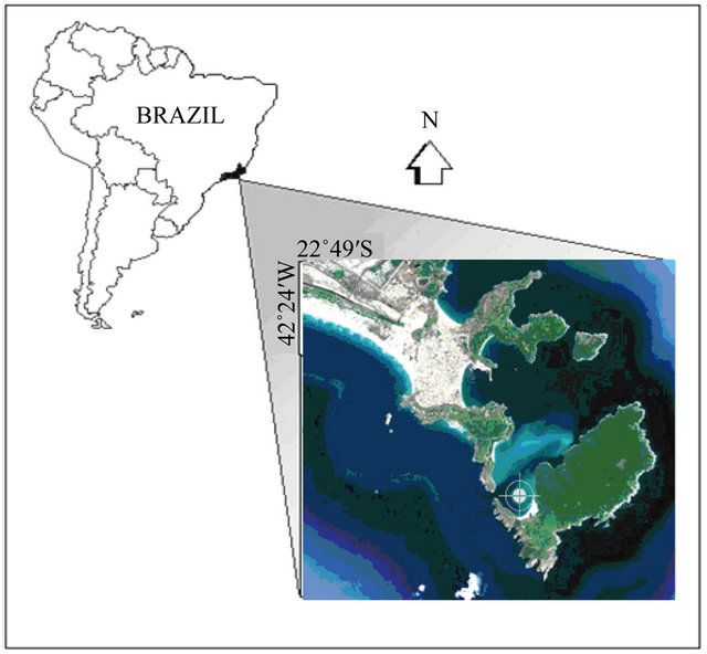
Figure 1. The Anjos embayment in Rio de Janeiro State, Brazil. The cycle indicates the sampling location.
the quantity and composition of the plankton communities, shifting the trophic structure.
2.2. Sampling Procedure
The physical and chemical data were provided by the oceanographic department of the Admiral Paulo Moreira Institute of Sea Studies (IEAPM) that maintain a seawater monitoring program with sampling once a week at the studied location. Samples are collected at surface (0.5 m depth) with a Nansen bottle and a coupled reverse thermometer outside. Salinity, oxygen and nutrients (PO4, NO2, NO3, NH4) are determined as described in [51] while meroplankton larvae (organism/m3) are collected by means drag plankton net of 100 mesh and counted under stereomicroscopy. To obtain correlations, we performed real time cytometric measurements of phytoplankton abundance and collected samples of 200 ml that were immediately fixed with 1% of formalin for further cytometric (~3 h) enumeration of bacterioplankton and viruses. The study started in August of 2006 and finished in June of 2007.
2.3. Flow Cytometry
Phytoplankton enumerations were performed in situ with the CytoBuoy flow cytometer (Cytobuoy b.v. Nieuwerbrug, The Netherlands). It is equipped with a solid blue laser providing 20 mW at 488 nm, one side scatter (SSC, 446/500 nm) detector and three others to detect red (chlorophyll-a) fluorescence (FL-1, 669/725 nm); orange/yellow (FL-2, 601/651) and green/yellow (FL-3, 515/585 nm) fluorescence respectively. The cytometer was left to run for 3 minute at a fixed flow rate of 2 m/s and the discriminator was set on SSC. Parameters were collected on a log scale using the CytoSift software and analyzed in the Cytowave software, both provided by the manufacturer.
Prokaryote enumeration were performed with a FACScan flow cytometer (Becton Dickson, San Jose, California) equipped with an air-cooled laser providing 15 mW at 488 nm and with the standard filter setup. To avoid clogging due to the small internal diameter of the sampling tube, all samples were primary filtered in 0.8 μm filters (Millipore). Yellow-green 0.92-µm beads (Fluoresbrite Microparticles, Polysciences) were added in the samples as internal standard. Bacterial samples were stained with SYBR-Green-1 at a final concentration of 0.5 × 10⁻⁴ of the commercial stock solution [10]. The samples were incubated for 15 min in the dark, the discriminator was set on green fluorescence, and the samples were analyzed for 1 min at a rate of 50 µL∙min–1.
For viral counts, we performed dilutions from 1:10 to 1:200 in TE buffer (10 mM Tris, 1 mM EDTA [pH 8.0]) to avoid coincidence and minimize the error due to lowvolume pipeting. These dilutions were heated at 80˚C for 10 min in the dark in the presence of SYBR-Green-1 at a final concentration of 0.5 × 10⁻⁴ and left to cool for 5 min according to [52]. The samples were analyzed in the FACScan flow cytometer at a delivery rate of 50 µL∙min–1. The cytometer was triggered to green fluorescence and the detection threshold was progressively decreased until viruses could be detected. All cytometric data were collected on a log scale and analyzed in the CellQuest™ Pro software provided by the manufacturer.
2.4. Artificial Neural Network
ANN is a data-driven model essentially composed of three interconnected layers of nodes called neurons: one “input layer” containing as many nodes as the analyzed parameters (in our case from FCM), a “hidden layer”, and one “output layer”. The input patterns (vectors) are presented to the input layer, which distributes this information to the hidden layer and the latter to the subsequent layer. In this study we were used, as ANN input, the cytometric data set related to counting of phytoplankton, bacterioplankton and their ratios. These data are not pre-processed. The data inputs were randomly split into 70% training, 20% testing and 10% validation [32,53].
The MLP-NN is a fully connected feedforward-type model that maps a set of input data onto a set of appropriate output. It was trained by the backpropagation learning technique [54] through the gradient descendent algorithm. In short, the training process involves the following basics steps:
1) The connection weights are assigned small, arbitrary values.
2) A training sample is presented to the network, producing a network output.
3) The global error function is calculated.
4) The connection weights (w) are adjusted using the gradient descent rule as:
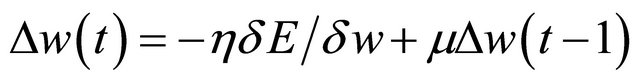 (1)
(1)
where h is the learning rate; m is the momentum value.
In RBF-NN [55], each node at the hidden layer represents a kernel or a separate basis function—a function for which the value depends solely on the distance between the input data and a fixed point, the center of the function, so that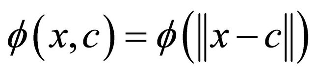 . Any function φ that satisfies the property
  is a radial function. Commonly the norm is usually the Euclidean distance. Radial basis functions are typically used to build up function approximations of the form:
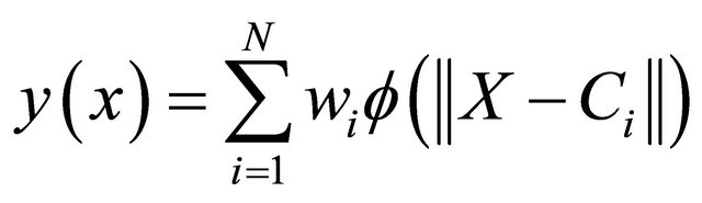 (2)
(2)
where the approximating function y(x) is represented as a sum of N radial basis functions, each associated with a different center Ci, and weighted by an appropriate coefficient wi. The weights wi are estimated using the matrix methods of linear least squares, because the approximating function is linear in the weights.
The GRNN [56] can only be used for regression problems based on nonparametric estimation [57]. It is closely related to a probabilistic neural network. Regression can be thought as the least-mean-square estimation of the value of a variable based on available data. This type of ANN is based on the estimation of a probability density function. It utilizes a probabilistic model between the independent vector random variable X with dimension D, and dependent scalar random variable Y, assuming that x and y are the measured values for the X and Y variables respectively. If f (x,Y) the known joint continuous probability density function, and if f (x,Y) is known, the expected value of Y given x (the regression of Y on x) can be estimated as:
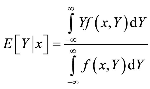 (3)
(3)
The first hidden layer in the GRNN contains radial units. A second hidden layer contains units that help to estimate the weighted average. This is a specialized procedure. Each output has a special unit assigned in this layer that forms the weighted sum for the corresponding output. To get the weighted average from the weighted sum, the weighted sum must be divided through by the sum of the weighting factors. A single special unit in the second layer calculates the latter value. The output layer then performs the actual divisions. In regression problems, typically only a single output is estimated, and so the second hidden layer usually has two units.
Finally, to measure the network performance, we used the typical root mean-square error (RMSE) expressed as:
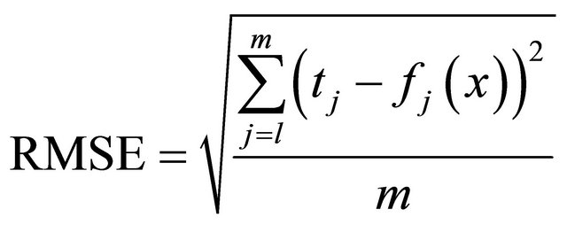 (4)
(4)
where m denotes the number of testing patterns.
2.5. Genetic Algorithm Optimization
A GA [58] is a search heuristic belonging to a class of evolutionary algorithms used for optimization problems whose techniques are inspired by natural evolution, such as inheritance, mutation, selection, and crossover [59]. Basically, a population of strings (called chromosomes) which encode candidate solutions (individual networks) to an optimization problem, evolve toward better solution. Figure 2 illustrates the simplest form of a GA that is usually implemented as the following algorithm:
1) Construct a random initial population. Individual solutions (called chromosomes);
2) Calculate and evaluate the fitness of each individual in the population;
3) Select the best ranking chromosomes for reproduce based on their fitness (higher);
4) Breed new generation applying crossover and/or mutation (genetic operators) and give birth the offspring;
5) Repeat from step two until a termination condition is reached (time limit or sufficient fitness achieved.
The power of GA derives largely from the concept of “implicit parallelism”, the simultaneous allocation of trials to many regions of the search space. The objective is the minimization of the error function with respect to the structure of the network the hidden node center and weights between hidden layer and output layer. The ANN configuration may then be formed as a multiobjective minimization problem whose objective function becomes a vector where J is defined as:
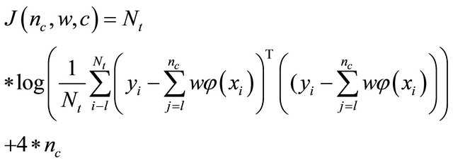 (5)
(5)
where Nt is the number of data samples in the training set, yi, xi are the output in the training and test set. The final product of GA is to obtain a neural architecture optimized to the subject studied.
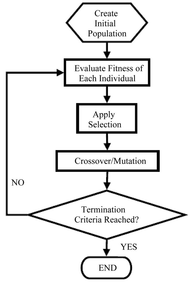
Figure 2. The flow chart of a general Genetic Algorithm. An example of a pseudo code relating to this flow chart can be found in [47].
3. Results and Discussion
Each dot depicted in Figure 3 is a suspended particle detected by the two cytometers. Figure 3(a), for example, presents the clusters of real time data of phytoplankton cells acquired by the CytoBuoy instrument since the red fluorescence signals are the results of chlorophyll-a response to the laser excitation and the side scatter (SSC) is proportional to cytoplasmic granularity of a cell or internal complexity measurement [60]. Individuals of these groups were better characterized by [39] at a single cell and species level. During the studied period, the total phytoplankton concentration varied from 3.30 × 10² cells/ml in the winter to 8.66 × 10² cells/ml in the summer.
On the other hand, Figure 3(b) shows the picoplankton particle distribution accessed by the FACScan flow cytometer. Three prokaryote clusters (HDNA-high DNA, LDNA-low DNA and G3 with different green fluorescence intensities are noted indicating different nucleic acid content. This distribution seems to be general and was found by other authors [4,5].
A recent study, in Arraial do Cabo upwelling region, characterized these communities as being dominated by Bacteroidetes phyla, Alphaproteobacteria class [61]. However, the three groups were quantified together to the purpose of this work and the total heterotrophs varied from 1.51 × 10³ cells/ml in the winter to 1.24 × 10⁶ cells/ml in the summer. Figure 3(b) show two viral populations which, according [2] are considered the major
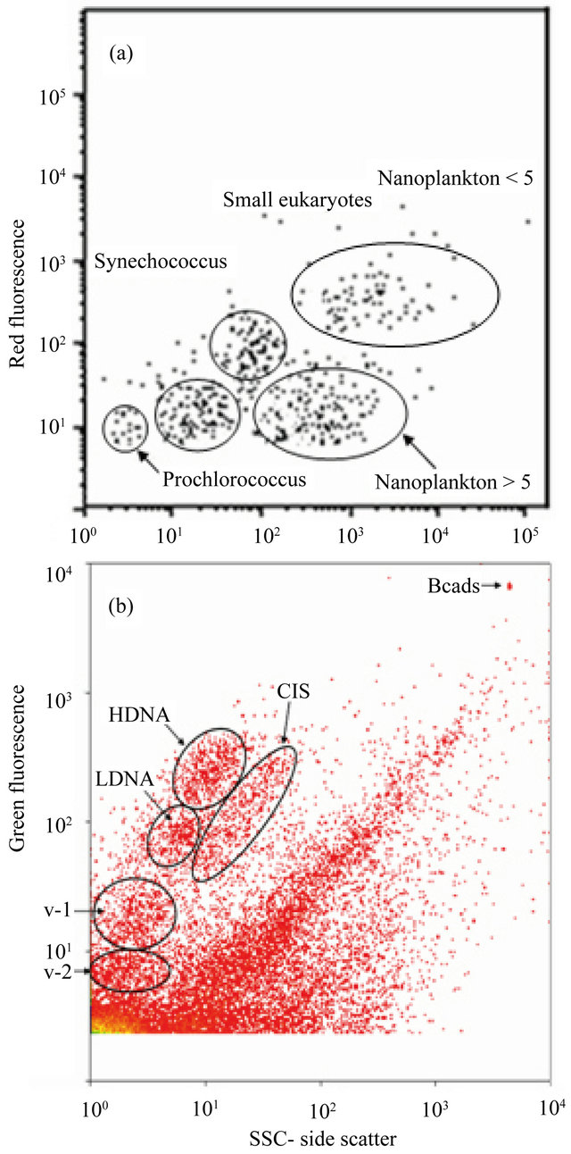
Figure 3. Flow cytometry detected groups. In (a), the in situ cytogram of the CytoBuoy instrument showing two cyanobacteria clusters another three of eukaryotes. In (b), it is presented three clusters of heterotrophic prokaryotes (HDNA, LDNA and G3) and two of marine viruses (V-1, V-2) related to a 1:50 sample dilution after staining.
causes of mortality and therefore the primary regulators of organismal abundance. While V-1 is a diverse group that infects the eukaryotic phytoplankton [10], V-2 are bacteriophages infecting prokaryotes. The total virus abundance varied from 6.21 × 10⁵ to 2.86 × 10⁶ during the studied period. Viruses were by far the most abundant biological entities, followed by heterotrophic prokaryotes, phytoplankton and meroplankton larvae. The latter category, collected by trawling plankton net, ranged in abundance from 9 to 1076.33 organisms/m3.
With a total of 39 field data acquisitions, the correlations among all studied variables are present in Table 1. In short the virioplankton community is highly correlated to heterotrophic prokaryotes (Het Prok) and phytoplankton (Phyto) cells but uncorrelated to the abiotic factors with exception to oxygen. However, the virus to bacterial ratio (VBR) indicates a negative correlation to heterotrophic prokaryotes (−0.33) and temperature (−0.36) while positive to NH4 (0.35), see Table 1. We call attention to the fact that VBR, which contain the prokaryotes as one of its components, can be related statistically to an autocorrelation. Together, these results led us to speculate at large we are looking to nitrifying process where virus could be involved indirectly. On the other hand, the prokaryote to phytoplankton ratio, the heterotrophs/ autotrophs balance, was found positive to heterotrophic prokaryotes and temperature what suggest that this system can be, at long term, a sink of carbon. An unexpected result is the meroplankton larvae that present a negative correlation to V-2 and positive to heterotrophic prokaryotes.
As previously reported by [7], the highest mean value of virioplankton occurred in SACW while the highest mean values of prokaryotes, phytoplankton and meroplankton larvae occurred in the mixing of coastal and tropical waters. The cold water of SACW showed the smallest Het Prok/Phyto ratio and the highest virus/bacterial ratio (VBR) indicating a great viral activity.
Figure 4 presents the temporal distribution of vireoplankton and temperature. It is possible to see a great variability the total virioplankton presenting the two higher values in the middle of the period. These peaks are coincident with low temperatures due to upwelling events. Although the lack of correlation between these two variables a seasonal behavior of virioplankton seems to emerge. Seasonality in virioplankton has been previously reported [62,63] but our data suggest a close relationship with upwelling process. The lack of correlation may be explained by the low sampling frequency or due to the sample size.
The solution obtained from the genetic algorithm to achieve the optimal ANN model followed the parameters below throughout the simulations:
• population size = 1500;
• crossover probability = 0.5 - method: roulette wheel selection;
• mutation probability = 0.1 - method of single point mutation and with bit string mutation technique;
• the networks were generated with a learning rate = 0.1, momentum = 0.3 and 500 cycles.
Figure 5 shows the behavior of the best three ANN models to estimate the abundance of viruses. In general all the three models are able to follow the behavior of this function however; the Multilayer Perceptron (MLP) neural network seems to be closer while Radial Basis Function (RBF) has a better estimation for higher values
Table 1. Spearman correlation of the variables: Temp refers to temperature as Sal to salinity, Virus to viruses, Het Prok to heterotrophic prokaryotes, Phyto is the total counts of autotrophs, VBR is the virus/bacterial ratio and Het/Aut is the heterotrophic/autotrophic ratio. Numbers, in bold, are statistically significant. Correlations are significant at p < 0.05000.
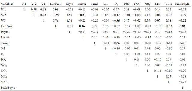
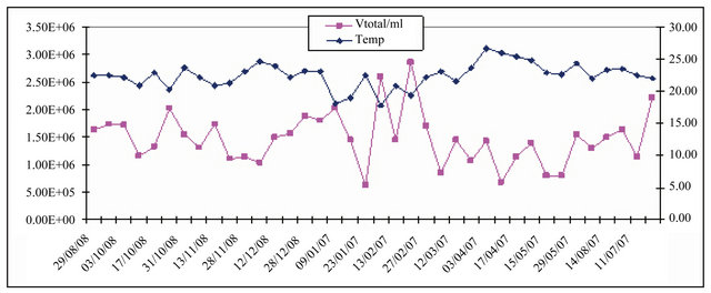
Figure 4. Temporal variation of the virioplankton community and temperature. The highest values of viruses concentration coincide with the smallest values of temperature.
(peaks) and the General Regression neural network (GRNN) for smaller ones. In our problem, we would like to get an optimized neural network architecture and minimum data set. This has been accomplished within 500 training cycles.
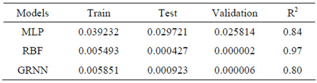
The Table 2 presents the RMSE of the training, test and validation data sets and the correlation coefficients (R2) to validation of the models. The RBF is the more fitted model (0.97) to perform this prediction but these results should be viewed with care due to RMSE penalize the error in the highest values. A detailed description of a RBF-NN generation and training is found in [64].
4. Conclusions
According [65], in lakes, and [66], in sea water, suggested that the quantity of viruses may reflect the trophic status of the ecosystem. It has also been proposed on several occasions that sediments can constitute a potentially important reservoir of infectious bacteriophages [67], cyanophages [68] or algal viruses [69]. However, no processes involving the recruitment of viruses into or their release from sediments had so far been clearly demonstrated. Previous studies have shown that viruses can be absorbed onto sinking particles, and thus carried down to the sea-floor [20] so that sediments receiving a high
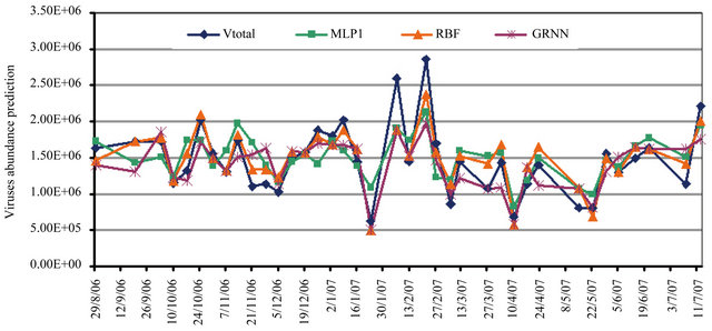
Figure 5. The three neural network models behavior to predict the total abundance of viruses (VT); MLP (Multilayer Perceptron), RBF (Radial Basis Function) and GRNN (General Regression Neural Network).
Table 2. Neural network performance and error (RMSE) in training, test and validation data set.
influx of particles might also receive large inputs of viruses from the water column. However, our data indicates that the upwelling process is likely to play a key role by producing the resuspension of virus like particles and organic matter through out the water column. During the up flow, environmental factors [70] such as temperature, and host biochemical features [71] may act as viral activation factors. In this way, the higher temperature and oligotrophic conditions of the coastal and tropical waters of the Arraial do Cabo upwelling system could be considered as ecological refuges resulting in a steady state that allows the co-existence of all populations.
The main goal was to free the network design process from constrains the humans biases, and discover better forms architectures. The automated search by GA method seems to be a good way to achieve this goal.
There are species of virus that can be predicted from their hosts. However, there are viruses of long spectrum that have multiple host and how we are working with all of them, we can not require a very accurate and precise results due to the uncertainties of the virus and host community. The neural networks model, in this work, proved to be capable of modeling a viral abundance in a water column. They are known as active biological agents and very important in marine food web. Thus, the main application of these models is the estimate of the virus to form more complex simulation models the dynamics of the energy flow between the various compartments planktonic, since the virus can not be accessed online.
Therefore, due to the complexity of the studied problem, we tried to develop a methodology that although with some limitations, it could to achieve satisfactory results to predict virioplankton abundance from cytometric data set.
5. Acknowledgements
The authors are grateful to Admiral Paulo Moreira Institute of Sea Studies experts for physical, chemical and meroplankton data and to the Brazilian Research Agencies (CAPES, CNPQ) for the financial support. Appreciation and thanks are also given to the anonymous reviewer for the constructive comments and suggestions to improve the manuscript.
REFERENCES
- C. P. D. Brussaard, S. W. Wilhelm, F. Thingstad, M. G. Weinbauer, G. Bratbak, M. Heldal, S. A. Kimmance, M. Middelboe, K. Nagasaki, J. H. Paul, D. C. Schroeder, C. A. Suttle, Vaqué and D. K. E. Wommack, “Global-Scale Processes with a Nanoscale Drive: The Role of Marine Viruses,” The ISME Journal, Vol. 2, 2008, pp. 1-4.
- C. A. Suttle, “Marine Viruses: Major Players in the Global Ecosystem,” Nature, Vol. 5, No. 8, 2007, pp. 801- 812.
- D. Lindell, J. D. Jaffe, M. L. Coleman, M. E. Futschik, I. M. Axmann, T. Rector, G. Kettler, M. B. Sullivan, R. Steen, W. R. Hess, G. M. Church and S. M. Chisholm, “Genome-Wide Expression Dynamics of a Marine Virus and Host Reveal Features of Co-Evolution,” Nature, Vol. 449, No. 7158, 2007, pp. 83-86. doi:10.1038/nature06130
- N. Jiao, Y. Zhao, T. W. Luo and X. Wang, “Natural and Anthropogenic Forcing on the Dynamics of Virioplankton in the Yangtze River Estuary,” Journal of Marine Biology Association United Kingdom, Vol. 86, No. 3, 2006, pp. 543-550. doi:10.1017/S0025315406013452
- J. P. Payet and C. A. Suttle, “Physical and Biological Correlates of Virus Dynamics in the Southern Beaufort Sea and Amundsen Gulf,” Journal of Marine Systems, Vol. 74, No. 3-4, 2007, pp. 933-945. doi:10.1016/j.jmarsys.2007.11.002
- J. L. Clasen, S. M. Brigden, J. P. Payet and C. A. Suttle, “Evidence That Viral Abundance across Oceans and Lakes Is Driven by Different Biological Factors,” Freshwater Biology, Vol. 53, No. 6, 2008, pp. 1090-1100. doi:10.1111/j.1365-2427.2008.01992.x
- G. C. Pereira, A. Granato, A. R. Figueiredo and N. F. F. Ebecken, “Virioplankton Abundance in Trophic Gradients of an Upwelling Field,” Brazilian Journal of Microbiology, Vol. 40, No. 4, 2009, pp. 857-865. doi:10.1590/S1517-83822009000400017
- O. Bergh, K. Y. Børsheim, G. Bratbak and M. Heldal, “High Abundance of Viruses Found in Aquatic Environments,” Nature, Vol. 340, 1989, pp. 467-468. doi:10.1038/340467a0
- R. T. Noble and J. A. Fuhrman, “Use of SYBR Green I for Rapid Epifluorescence Counts of Marine Viruses and Bacteria,” Aquatic Microbial Ecology, Vol. 14, No. 2, 1998, pp. 113-118. doi:10.3354/ame014113
- D. Marie, C. P. D. Brussaard, R. Thyrhaug, G. Bratbak and D. Vaulot, “Enumeration of Marine Viruses in Culture and Natural Samples by Flow Cytometry,” Applied and Environmental Microbiology, Vol. 65, No. 1, 1999, pp. 45-52.
- Y. Bettarel, T. Sine-Nagano, C. Amblard and H. Laveran, “A Comparison of Methods for Counting Viruses in Aquatic Systems,” Applied and Environmental Microbiology, Vol. 66, No. 6, 2000, pp. 2283-2289. doi:10.1128/AEM.66.6.2283-2289.2000
- M. M. Ferris, C. L. Stoffel, T. T. Maurer and K. L. Rowlen, “Quantitative Intercomparison of Transmission Electron Microscopy, Flow Cytometry, and Epifluorescence Microscopy for Nanometric Particle Analysis,” Analytical Biochemistry, Vol. 304, No. 2, 2002, pp. 249-256. doi:10.1006/abio.2002.5616
- C. Courties, A. Vaquer, M. Tousselier, M. J. ChretiennotDinet, J. Neveux, C. Machado and H. Claustre, “Smallest Eukaryotic Organism,” Nature, Vol. 370, No. 255, 1994. p. 255.
- M. Yanada, T. Yokokawa, C. H. Lee, H. Tanaka, I. Kudo and Y. Maita, “Seasonal Variation of Two Different Heterotrophic Bacterial Assemblages in Subarctic Coastal Seawater,” Marine Ecology Progress Series, Vol. 204, 2000, pp. 289-292. doi:10.3354/meps204289
- E. S. Lindström, T. Weisse and P. Sadler, “Enumeration of Small Ciliates in Culture by Flow Cytometry and Nucleic Acid Staining,” Journal Microbiological Methods, Vol. 49, No. 2, 2002, pp. 173-182. doi:10.1016/S0167-7012(01)00366-9
- J. M. Rose, D. A. Caron, M. E. Sieracki and N. Poulton, “Counting Heterotrophic Nanoplanktonic Protists in Cultures and Aquatic Communities by Flow Cytometry,” Aquatic Microbial Ecology, Vol. 34, No. 3, 2004, pp. 263-277. doi:10.3354/ame034263
- G. B. J. Dubelaar and P. L. Gerritzen, “CytoBuoy: A Step Forward towards Using Flow Cytometry in Operational Oceanography,” Scientia Marina, Vol. 64, No. 2, 2000, pp. 255-265.
- R. J. Olson, A. Shalapyonok and H. M. Sosik, “An Automated Submersible Floe Cytometer for Analyzing Pico and Nanoplankton: FlowCytobot,” Deep-Sea Research I, Vol. 50, No. 2, 2003, pp. 301-315. doi:10.1016/S0967-0637(03)00003-7
- R. Danovaro, A. Dellanno, A. Trucco, M. Serresi and S. Vanucci, “Determination of Viruses in Marine Sediments,” Applied and Environmental Microbiology, Vol. 67, No. 3, 2001, pp. 1384-1387. doi:10.1128/AEM.67.3.1384-1387.2001
- I. Hewson and J. A. Fuhrman, “Viriobenthos Production and Virioplankton Sorptive Scavenging by Suspended Sediment Particles in Coastal and Pelagic Waters,” Microbiological Ecology, Vol. 46, No. 3, 2003, pp. 337-347. doi:10.1007/s00248-002-1041-0
- M. S. Schwalbach, I. Hewson and J. A. Fuhrman, “Viral Effects on Bacterial Community Composition in Marine Plankton Microcosms,” Aquatic Microbial Ecology, Vol. 34, No. 2, 2004, pp. 117-127. doi:10.3354/ame034117
- D. Prangishvili, P. Forterre and R. A. Garrett, “Viruses of the Archaea: A unifying view,” Nature Reviews Microbiology, Vol. 4, No. 11, 2006, pp. 837-48. doi:10.1038/nrmicro1527
- A. C Baudoux and C. P. Brussaard, “Characterization of Different Viruses Infecting the Marine Harmful Algal Bloom Species Phaeocystis globosa,” Virology, Vol. 341, No. 1, 2005, pp. 80-90. doi:10.1016/j.virol.2005.07.002
- Y. Takao, K. Nagasaki, K. Mise, T. Okuno and D. Honda, “Isolation and Characterization of a Novel Single-Stranded RNA Virus Infectious to a Marine Fungoid Protist, Schizochytrium sp. (Thraustochytriaceae, Labyrinthulea),” Applied and Environmental Microbiology, Vol. 71, No. 8, 2004, pp. 4516-4522. doi:10.1128/AEM.71.8.4516-4522.2005
- M. G. Fischer, M. J. Allen, W. H. Wilson and C. A. Suttle, “Giant Virus with a Remarkable Complement of Genes Infects Marine Zooplankton,” Proceedings National Academy Science, Vol. 107, No. 45, 2010, pp. 19508-19513. doi:10.1073/pnas.1007615107
- J. Zhuang, G. Cai, Q. Lin, Z. Wu and L. Xie, “A Bacteriophage-Related Chimeric Marine Infecting Abalone,” PloS ONE, Vol.5, No. 11, 2010, pp. 1-12. doi:10.1371/journal.pone.0013850
- A. Vardi, B. A. S. Van Mooy, H. F. Fredricks, K. J. Popendorf, J. E. Ossolinski, L. Haramaty and K. D. Bidle, “Viral Glycosphingolipids Induce Lytic Infection and Cell Death in Marine Phytoplankton,” Science, Vol. 326, No. 5954, 2009, pp. 861-865. doi:10.1126/science.1177322
- A. Long, L. D. McDaniel, J. Mobberley and J. H. Paul, “Comparison of Lysogeny (Prophage Induction) in Heterotrophic Bacterial and Synechococcus Populations in the Gulf of Mexico and Mississippi River Plume,” The ISME Journal, Vol. 2, 2008, pp. 132-144. doi:10.1038/ismej.2007.102
- D. Coombs, M. A. Gilchrist, J. Percus and A. S. Perelson, “Optimal Viral Production,” Bulletin of Mathematical Biology, Vol. 65, No. 6, 2003, pp. 1003-1023. doi:10.1016/S0092-8240(03)00056-9
- K. E. Wommack and R. R. Colwell, “Virioplankton: Viruses in Aquatic Ecosystems,” Microbiology and Molecular Biology, Vol. 64, No. 1, 2000, pp. 69-114. doi:10.1128/MMBR.64.1.69-114.2000
- M. Middelboe, “Bacterial Growth Rate and Virus-Host Dynamics,” Microbial Ecology, Vol. 40, No. 2, 2000, pp. 114- 124.
- S. Haykin, “Neural Networks,” Prentice Hall, Upper Saddle River, 1999
- M. Scardi, “Artificial Neural Network as Empirical Models of Phytoplankton Production,” Marine Ecological Progress Series, Vol. 139, 1996, pp. 289-299. doi:10.3354/meps139289
- R. S. Woodd-Walkers, K. S. Kingston and C. P. Gallienne, “Using Neural Networks to Predict Surface Zooplankton Biomass along a 50˚N to 50˚S Transect of the Atlantic,” Journal of Plankton Research, Vol. 23, No. 8, 2001, pp. 875-888. doi:10.1093/plankt/23.8.875
- G. Brion, C. Viswanathan, T. R. Neelakantan, S. Lingireddy, R. Girones, D. Lees, A. Allard and A. Vantarakis, “Artificial Neural Network Prediction of Viruses in Shellfish,” Applied and Environmental Microbiology, Vol. 71, No. 9, 2005, pp. 5244-5253. doi:10.1128/AEM.71.9.5244-5253.2005
- J. D. Olden, N. L. Poff and B. P. Bledsoe, “Incorporating Ecological Knowledge into Ecoinformatics: An Example of Modeling Hierarchically Structured Aquatic Communities with Neural Network,” Ecological Informatics, Vol. 1, No. 1, 2006, pp. 33-42. doi:10.1016/j.ecoinf.2005.08.003
- Tae-Soo, I. S. Kawak and Y. S. Park, “Patterns Recognition of Long-Term Ecological Data in Community Changes by Using Artificial Neural Network: Benthic Macroinvertebates and Chironomids in a Polluted Stream,” Korean Journal Ecology, Vol. 23, No. 2, 2000, pp. 89-100.
- S. Malek, A. SalleH and M. S. Baba, “Analysis of Selected Algal Growth (Pyrrophyta) in Tropical Lake Using Kohonen Self Organizing Feature Map (SOM) and Its Prediction Using Rule Based Systems,” International Conference and Workshop on Emerging Trends on Technology, Mumbai, 26-27 February 2010, pp. 761-764. doi:10.1145/1741906.1742083
- G. C. Pereira and N. F. F. Ebecken, “Combining in Situ Flow Cytometry and artificial Neural Networks for Aquatic Systems Monitoring,” Expert Systems with Applications, Vol. 38, No. 8, 2011, pp. 9626-9632. doi:10.1016/j.eswa.2011.01.140
- G. Yen and H. Lu, “Hierarchical Genetic Algorithm for near Optimal Feedforward Neural Network Design,” International Journal Neural Systems, Vol. 12, No. 1, 2002, pp. 31-43.
- Z.-Y. Xing, Y. Zhang, Y. Qin, L.-M. Jia and Y.-Y. Wu, “A Hierarchical Genetic Algorithm Based RBF Neural Network Approach for Modelling of Electrohydraulic System,” ICROS-SICE International Joint Conference, Fukuoka International Congress Center-Japan, 18-21 August 2009.
- R. Ghorbani, Q. Wu and G. G. Wang, “Nearly Optimal Neural Network Stabilization of Bipedal Standing Using Genetic Algorithm,” Engineering Applications of Artifi- cial Intelligence, Vol. 20, No. 4, 2007, pp. 473-480. doi:10.1016/j.engappai.2006.09.007
- S. H. Ling and F. H. F. Leung, “An Improved Genetic Algorithm with Average-Bound Crossover and Wavelet Mutation Operations,” Soft Computing, Vol. 11, No. 1, 2007, pp. 7-31. doi:10.1007/s00500-006-0049-7
- N. Öztürk, “Use of Genetic Algorithm to Design Optimal Neural Network Structure,” Engineering Computations, Vol. 20, No. 8, 2003, pp. 979-997. doi:10.1108/02644400310502982
- S. H. Ling, “A New Neural Network Structure: Node-toNode-Link Neural Network,” Journal of Intelligence Learning Systems and Application, Vol. 2, No. 1, 2010, pp. 1-11. doi:10.4236/jilsa.2010.21001
- S. H. Ling and H. K. Lam, “Playing Tic-Tac-Toe Using Genetic Neural Network with Double Transfer Functions,” Journal of Intelligence Learning Systems and Application, Vol. 3, No. 1, 2011, pp. 37-44. doi:10.4236/jilsa.2011.31005
- F. H .F. Leung, H. K. Lam, S. H. Ling and P. K. S. Tam, “Tuning of the Structure and Parameters of Neural Network Using an Improved Genetic Algorithm,” IEEE Transactions on Neural Networks, Vol. 14, No. 1, 2003, pp. 79-88. doi:10.1109/TNN.2002.804317
- S. A. Gaeta, J. A. Lorenzetti, L. B. Miranda, S. M. M. Susimi-Ribeiro, M. Pompeu and C. E. S. Araújo, “The Vitória Eddy and Its Relation to the Phytoplankton Biomass and Primary Production during the Austral Fall of 1995,” Archive Fishery Marine Research, Vol. 47, No. 2-3, 1999, pp. 253-270.
- G. C. Pereira, R. Coutinho and N. F. F. Ebecken, “Data Mining for Environmental Analysis and Diagnostic: A Case Study of Upwelling Ecosystem of Arraial do Cabo,” Brazilian Journal of Oceanography, Vol. 65, No. 1, 2008, pp. 1-12. doi:10.1590/S1679-87592008000100001
- M. Guenther, E. Gonzalez-Rodriguez, W. F. Carvalho, C. E. Rezende, G. Mugrabe and J. L. Valentin, “Plankton Trophic Structure and Particulate Organic Carbon Production during a Coastal Downwelling-Upwelling Cycle,” Marine Ecololy Progress Series, Vol. 363, 2008, pp. 109-119. doi:10.3354/meps07458
- SCOR, “Protocols for the Joint Global Ocean Flux Study (JGOFS) Core Measurements,” Scientific Committee on Ocean Research, International Council of Scientific Unions 9170, Bergen, 1996.
- C. P. D. Brussaard, “Optimization of Procedures for Counting Viruses by Flow Cytometry,” Applied and Environmental Microbiology, Vol. 70, No. 3, 2004, pp. 1506-1513. doi:10.1128/AEM.70.3.1506-1513.2004
- M. Kearns, “A Bound on the Error of Cross Validation Using the Approximation and Estimation Rates, with Consequences for the Training-Test Split,” AT&T Research, Murray Hill, 1996, pp. 183-189.
- D. E. Rumelhart, G. E. Hinton and R. J. Williams, “Learning Representations by Back-Propagation Error,” Nature, Vol. 323, 1986, pp. 533-536. doi:10.1038/323533a0
- M. D. Buhmann, “Radial Basis Functions: Theory and Implementations,” Cambridge University Press, Cambridge, 2003. doi:10.1017/CBO9780511543241
- D. F. Specht, “A General Regression Neural Network,” IEEE Transactions on Neural Networks, Vol. 2, 1991, pp. 568-1989. doi:10.1109/72.97934
- L. Rutkowski, “Generalized Regression Neural Network in Time-Varying Environment,” IEEE Transactions on Neural Networks, Vol. 15, No. 3, 2004, pp. 576-596. doi:10.1109/TNN.2004.826127
- J. H. Holland, “Adaptation in Natural and Artificial Systems,” University of Michigan Press, Ann Abor, 1975.
- D. E. Goldberg, “Genetic Algorithm in Search, Optimization, and Machine Learning,” Addison-Wesley, New York, 1989.
- [61] G. Salzmann, “Light Scatter: Detection and Usage,” Current Protocols in Cytometry, No. 9, 1999. doi:10.1002/0471142956
- [62] J. C. Cury, F. V. Araujo, S. A. Coelho-Souza, R. S. Peixoto, J. A. L. Oliveira, H. F. Santos, A. M. R. Dávila and A. S. Rosado, “Microbial Diversity of a Brazilian Coastal Region Influenced by an Upwelling System and Anthropogenic Activity,” PloS ONE, Vol. 6, No. 1, 2011, pp. 1-13. doi:10.1371/journal.pone.0016553
- [63] J. C. Auguet, H. Montanie, D. Delmas, H. J. Hartmann, and V. Huet, “Dynamic of Virioplankton Abundance and Its Enviromental Control in the Charente Estuary (France),” Microbial Ecology, Vol. 50, No. 3, 2005, pp. 1-13. doi:10.1007/s00248-005-0183-2
- [64] S. J. Williamson, L. A. Houchin, L. Daniel and J. H. Paul, “Seasonal Variation in Lysogeny as Described by Prophage Induction in Tampa Bay, Florida,” Applied and Environmental Microbiology, Vol. 68, No. 9, 2002, pp. 4307-4314. doi:10.1128/AEM.68.9.4307-4314.2002
- [65] A. Barreto, H. Barbosa and N. F. F. Ebecken, “Growing Compact RBF Networks Using a Genetic Algorithm,” Proceedings of the 7th Brazilian Symposium on Neural Networks, São Luís, 11-14 November 2002.
- [66] A. Conty, F. Garcia-Criado and E. Bécares, “Changes in Bacterial and Ciliate Densities with Trophic Status in Mediterranean Shallow Lakes,” Hydrobiologia, Vol. 584, No. 1, 2007, pp. 327-335. doi:10.1007/s10750-007-0585-x
- [67] M. G. Weinbauer, D. Fuks and P. Peduzzi, “Distribution of Viruses and Dissolved DNA along a Coastal Trophic Gradient in the Northern Adriatic Sea,” Applied and Environmental Microbiology, Vol. 59, No. 12, 1993, pp. 4074-4082.
- [68] M. Breitbart, B. Felts, S. Kelley, J. M. Mahaffy, J. Nulton, P. Salomon and F. Rohwer, “Diversity and Population Structure of a Near-Shore Marine-Sediment Viral Community,” Proceedings of the Royal Society B: Biological Sciences, Vol. 271, No. 1539, 2003, pp. 565-574.
- [69] M. G. Weinbauer, “Ecology of Procaryotic Viruses,” FEMS Microbiology Reviews, Vol. 28, No. 2, 2004, pp. 127-181. doi:10.1016/j.femsre.2003.08.001
- [70] K. Nagasaki, Y. Shirai, Y. Tomaru, K. Nishida and S. Pietrokovski, “Algal Viruses with Distinct Intraspecies Host Specificities Include Identical Intein Elements,” Applied and Environmental Microbiology, Vol. 71, No. 7, 2005, pp. 3599-3607. doi:10.1128/AEM.71.7.3599-3607.2005
- [71] L. McDaniel and J. H. Paul, “Effect of Nutrient Addition and Environmental Factors on Prophage Induction in Natural Populations of Marine Synechococcus Species,” Applied and Environmental Microbiology, Vol. 71, No. 2, 2005, pp. 842-850. doi:10.1128/AEM.71.2.842-850.2005
- [72] K. D. Bidle, L. Haramaty, J. Barcelos e Ramos and P. Falkowski, “Viral Activation and Recruitment of Metacaspases in the Unicellular Coccolithophore, Emiliania huxleyi,” Proceedings National Academy Science, Vol. 104, No. 14, 2007, pp. 6049-6054. doi:10.1073/pnas.0701240104
NOTES
*Corresponding author.