Journal of Water Resource and Protection
Vol.07 No.15(2015), Article ID:60482,15 pages
10.4236/jwarp.2015.715101
Contribution to the Analytical Equation Resolution Using Charts for Analysis and Design of Cylindrical and Conical Open Surge Tanks
Aboudou Seck1*, Musandji Fuamba2
1Department of Civil, Geological and Mining Engineering, Polytechnique Montréal, 2500 Chemin de Polytechnique, Montreal, QC, Canada
2Department of CGEM, Polytechnique Montréal, Succursale Centre, Montréal, Canada
Email: *aboudou.seck@polymtl.ca
Copyright © 2015 by authors and Scientific Research Publishing Inc.
This work is licensed under the Creative Commons Attribution International License (CC BY).
http://creativecommons.org/licenses/by/4.0/


Received 2 September 2015; accepted 19 October 2015; published 22 October 2015
ABSTRACT
In the event of an instantaneous valve closure, the pressure transmitted to a surge tank induces the mass fluctuations that can cause high amplitude of water-level fluctuation in the surge tank for a reasonable cross-sectional area. The height of the surge tank is then designed using this high water level mark generated by the completely closed penstock valve. Using a conical surge tank with a non-constant cross-sectional area can resolve the problems of space and height. When addressing issues in designing open surge tanks, key parameters are usually calculated by using complex equations, which may become cumbersome when multiple iterations are required. A more effective alternative in obtaining these values is the use of simple charts. Firstly, this paper presents and describes the equations used to design open conical surge tanks. Secondly, it introduces user-friendly charts that can be used in the design of cylindrical and conical open surge tanks. The contribution can be a benefit for practicing engineers in this field. A case study is also presented to illustrate the use of these design charts. The case study’s results show that key parameters obtained via successive approximation method required 26 iterations or complex calculations, whereas these values can be obtained by simple reading of the proposed chart. The use of charts to help surge tanks designing, in the case of preliminary designs, can save time and increase design efficiency, while reducing calculation errors.
Keywords:
Hydraulic Transients, Surge Tank, Water Hammer, First-Order Non-Homogeneous Differential Equation with Variables Coefficients, Friendly Charts

1. Introduction
A water hammer is defined as a pressure surge or wave caused when a fluid in motion is suddenly forced to stop or change directions. Water hammers usually occur when the flow of water into a turbine or pump decreases rapidly due to a sudden drop in the pressure head, or when a valve is suddenly closed at an end of a pipeline system. This creates a pressure wave that propagates through the pipe: this phenomenon in the pipe is called a penstock. In order to remedy such a situation, a surge tank can be connected to the piping system which (depending on the number of tanks, arrangement, and the nature of the restriction between the surge tank and the piping system) can take several forms and configurations. Besides the simple cylindrical surge tank, other types are adopted: conical surge tank, surge tank with internal bell-mouthed spillway, differential surge tank, etc. [1] . The design of open surge tank requires the solving of first-order, non-homogeneous, linear differential equations. This process will lead to an implicit equation for the determination of key parameters of a surge tank and the penstock. The solution will be found either by using an equation solver or by trial and error.
For preliminary designs, practicing engineers are usually overwhelmed with all the details of pipeline or canal systems. They need the general framework to build the surge tank in hydroelectric power plants projects. Simplified charts may help to facilitate identification of key parameters and variations.
Basically, the origin of the theory of water hammer goes back to the contributions of Menabrea [2] , who published a short note on the calculation of water pressures [3] . However, by its mathematical rigor and significant theories, the papers of Michaud [4] and [5] , Allievi [6] , [7] and [8] , Schnyder [9] and Jaeger [10] are the source of inspiration for all studies on water hammer. The use of surge tanks in hydropower systems and their problems with stability were reviewed by Lescovich [11] , Roche [12] and Chaudhry [13] (with extensive bibliography on this subject, where significant theories are found in Jaeger [14] [15] ).
Guinot [16] focuses on theoretical and practical implementation of Godunov approach to simulate the water hammer with steady friction, which induces a non-hyperbolic source term. But for transient flow in a constant diameter pipe, the friction factor which is the sum of the quasi-steady part and unsteady part, is developed in the model by Brunone et al. [17] , and modified by Bergant et al. [18] .
Research by Chaudhry et al. [19] , Finnemore et al. [20] and Moghaddam [21] provided analytical implicit equations for analysing and designing a simple surge tank. These equations yielded cylindrical surge tank dimensions that were solved either numerically or by trial and error. However, using these equations required long computational times.
Chaudhry et al. [22] investigated the stability of water level oscillations inside a closed surge tank during transient conditions. The result of this investigation led them to obtain stability diagrams which helped to indicate the demarcation of stable, unstable and incompatible regions within a closed surge tank. Though significant contributions dating back to the 1950’s had helped designers to better understand the behaviours of a surge tank, no diagrams were ever developed for reference purposes in the designing of cylindrical and conical surge tanks.
The impact of the presence of a surge tank on a pipeline system was added to the research by Kim [23] through the application of a Genetic Algorithm (GA) into the Impulse Response method platform, which derived the impedance functions for pipeline systems equipped with a surge tank. In his quest to secure a set of global optimum parameter values for a surge tank (such as location along the pipeline, the length of the connector, and the diameters required for the connector and the surge tank), Kim utilized four different objective functions and 2500 iterations with identical GA input parameters. However, to solve an example of a simple case application, Kim required 1250 iterations before obtaining the global optimum parameter values.
Ramadan et al. [24] investigated the effects of different key parameters on surge tank designs, such as the friction losses coefficient, surge tank cross-sectional area on the water surface, oscillations tank, and total discharge. The design analysis was tested under steady conditions. Unfortunately, their study is considered restrictive as their model does not allow for surge tank analysis or design in steady hydraulic system conditions, with initial input data other than those provided in their study.
All of these contributions require sophisticated resolution models and a long processing time. This paper bridges the gap between the design concept and the detailed design phase on surge tanks by providing user- friendly diagrams for the design of cylindrical and conical open surge tanks.
2. Methodology
This paper focuses on analytical approach to the unsteady flow of incompressible fluid in pipes. The non-con- stant cross-sectional area of surge tanks induces the first-order non-homogeneous differential equation with variable coefficients of water hammer. Firstly, the governing equations are derived; secondly charts for analysis and design of cylindrical and conical open surge tanks are given; and finally, one case study is presented and a comparative study between the successive approximation method and the resolution by the charts is done.
3. Governing Equations
Figure 1 presents sketches that define a surge tank analysis in three different flow scenarios: steady flow conditions, transient flow conditions, and conditions at the end of a time interval (after the closing of the valve).
3.1. First-Order Non-Homogeneous Differential Equation ODE with Variable Coefficients
In steady flow conditions, the difference Z0 in water level between the static level of the reservoir and the surge tank (measured negatively downward from the static water level) is equal to the sum of the head loss due to velocity head, friction, and any minor losses in the pipe as represented by Equation (1).
 (a)
(a) (b)
(b) (c)
(c)
Figure 1. Definition sketch for surge tank analysis. (a) Steady condition (initially); (b) The conditions in a time interval before the total closures of the valve; (c) The conditions at the end of the time interval.
 (1)
(1)
where
 (2)
(2)
Transient flow conditions occur at a time interval prior to total valve closure and are characterized by Equation (3), where dZ/dt represents the flow velocity through the surge tank when the valve is completely closed.
 (3)
(3)
The conditions at the end of time interval are characterized by the continuity as in Equation (4).
 (4)
(4)
where,
 (5)
(5)
And
 (6)
(6)
As a result, Equation (5) becomes
 (7)
(7)
Substituting Equation (7) into Equation (4), and rearranging Equation (3) gives the first-order non-homoge- neous differential equation with variable coefficients, where the non-constants coefficients b and c are continuous functions of Z.
 (8)
(8)
where,
 (9)
(9)
With
 (10)
(10)
3.2. Solution of ODE
The solution of Equation (8) is the sum of a particular solution and the general solution of the associated homogeneous equation .
.
Solving by integration and isolating X leads to a family of solutions associated to the homogeneous equation:
 (11)
(11)
This general solution (Equation (11)) contains a constant of integration λ, which denotes any real number. One particularity of homogeneous linear differential equations is that X = 0 represent a solution called the trivial solution. However, solutions of interest for this paper fall under the category of non-trivial solutions. Particular solution by variation of parameters is used [25] . This particular solution is expressed in the following terms:
 (12)
(12)
where,
 (13)
(13)
 (14)
(14)
 (15)
(15)
 (16)
(16)
Finally, the general solution of the non-homogeneous equation is obtained:
 (17)
(17)
Or, since X = V2, the general equation relating the velocity V in the pipe to the water surface level Z in the conical surge tank is:
 (18)
(18)
The unknown constant of integration λ is eliminated with the initial conditions (Equation (1): when V = V0 then Z = Z0) and the final conditions (when V = 0 then Z = Zmax).
3.3. Solving ODE with Initial-Value and Final-Value Constraints
・ For initial conditions, substituting these into Equation (18) and rearranging gives:
 (19)
(19)
where
 (20)
(20)
 (21)
(21)
 (22)
(22)
 (23)
(23)
 (24)
(24)
・ For final conditions, substituting these into Equation (18) and rearranging gives:
 (25)
(25)
where
 (26)
(26)
 (27)
(27)
 (28)
(28)
 (29)
(29)
 (30)
(30)
Finally, dividing Equation (25) by Equation (19) gives:
 (31)
(31)
Multiplying the numerator and denominator of the left-hand side of Equation (31) by K produces a result that leads to an implicit equation for all parameters Z0, V0, Zmax, K, L, DS0, m and DS:
 (32)
(32)
where
 (33)
(33)
 (34)
(34)
 (35)
(35)
 (36)
(36)
 (37)
(37)
 (38)
(38)
 (39)
(39)
 (40)
(40)
 (41)
(41)
 (42)
(42)
 (43)
(43)
However, solving Equation (32) for Z0, V0, Zmax, K, L, DS0, m or DS requires an equation solver or manual trial and error.
Another method is to first find Zmax = Zm for M = 0 (corresponding to a cylindrical or simple surge tank) using Equation (44) and then find  with M ≠ 0 (corresponding to the conical surge tank) using Equation (45).
 (44)
(44)
 (45)
(45)
Equations (32), (44) and (45) are based on four parameters Y, W, M and Zmax.
From Equations (44) one can show that:
 (46)
(46)
4. Charts
The charts, which are presented in Figures 2-11, relate maximum level of the water surface in the surge tank

Figure 2. Graph of Zmax vs. W for M = 0.

Figure 3. Graph of Zmax vs. W for M = 0.001.

Figure 4. Graph of Zmax vs. W for M = 0.01.
and parameters Y and W for fully developed flow. These charts represent the solutions of the Equations (32), (44) and (45) for values of M ranging from 0 to 0.3 and for values of Y lower than 40 meters.

Figure 5. Graph of Zmax vs. W for M = 0.02.
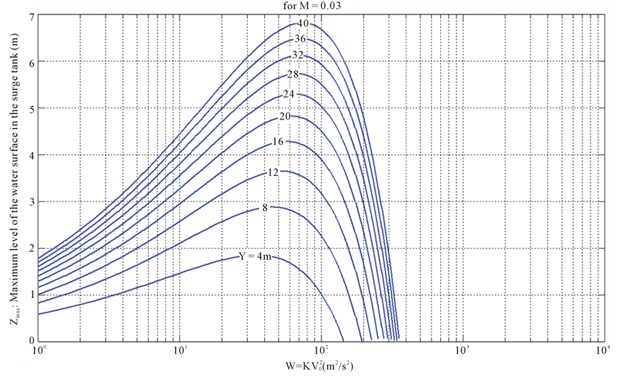
Figure 6. Graph of Zmax vs. W for M = 0.03.
5. Case Study
5.1. Application Examples
All case study problems have been derived from Finnemore et al. [20] . This reference is well known and well respected in the civil engineering field.

Figure 7. Graph of Zmax vs. W for M = 0.04.
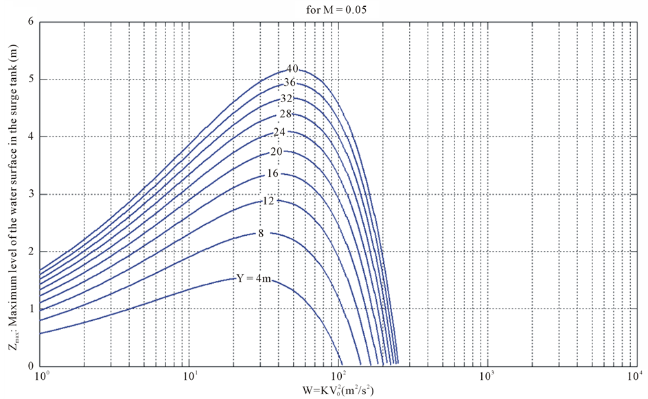
Figure 8. Graph of Zmax vs. W for M = 0.05.
・ Problem 1 (Figure 1(a)): A 42-in diameter steel pipe MN 3600 ft long (flush inlet, ƒ = 0.017) supplies water to a small power plant. The discharge (Q) = 200 cfs, the entrance loss coefficient ke = 0.5, JN = 100 ft, and

Figure 9. Graph of Zmax vs. W for M = 0.1.

Figure 10. Graph of Zmax vs. W for M = 0.2.
the elevations of J and the valve N are respectively 130 ft and 145 ft below the reservoir water surface. To protect against an instantaneous valve closure, what height would be required for a simple 6.5 ft diameter
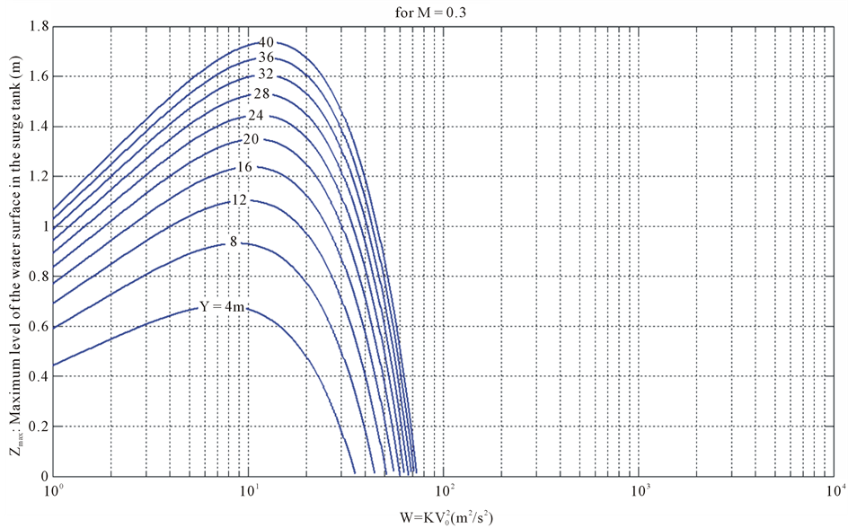
Figure 11. Graph of Zmax vs. W for M = 0.3.
surge tank in order for it to not overflow? In the surge tank only, neglect the velocity head, minor losses, fluid friction, and inertial effects.
・ Problem 2: Recalculate Problem 1 using the same parameters, while also neglecting velocity head and minor losses in the pipeline.
・ Problem 3: Recalculate Problem 1 using a surge tank diameter of 10 ft.
・ Problem 4: Using the data found in Problem 1, calculate the diameter of the surge tank that will require a tank height of 165 ft to prevent surge overflow.
・ Problem 5: Using the parameters in Problem 2, calculate the diameter of surge tank that produce a surge requiring a tank height of 165 ft.
Problems above have been solved by using two (2) methods: successive approximation and using the charts presented in this paper. The aim of this exercise is to evaluate the precision and speed of applying our charting solutions versus using the successive approximation method.
5.2. Solutions Using Charts versus by Successive Approximation Method
・ Problem 1:
Using charts:
Original data: Q = 200 cfs = 5.663 m3/s; ƒ = 0.017; ke = 0.5; m = 0 (simple surge tank); D = 42 in = 1.067 m; Ds0 = 6.5 ft = 1.981 m; L = MJ = 3600 ? 100 = 3500 ft = 1066.8 m; V0 = 4Q/(πD2) = 6.34 m/s;
The elevation of J is 130 ft = 39.62 m.
Using the equations listed below, the following values can be derived:
From Equation (2): K = 18.5
From Equation (6): Ds = 1.981 m
From Equation (41): W = 743.6 m2/s2
From Equation (42): Y = 16.72 m
From Equation (43): M = 0
And from Equation (46): 
So by plotting values M, W and Y on Figure 2, one finds that: Zmax = 16.00 m;
Height of surge tank = 39.62 + 16.00 = 55.62 m
Finnemore et al. [20] , by using successive approximation method, found Zmax = 16.05 m and the height of surge tank = 55.68 m after 6 iterations.
・ Problem 2:
Using charts:
By neglecting the velocity head and minor losses in the pipeline, K = 17
Using the equations listed below, the following values are derived:
From Equation (41): W = 683.3 m2/s2
From Equation (42): Y = 18.21 m
From Equation (46): 
So, again, by plotting values M, W and Y on Figure 2, one finds that: Zmax = 17.25 m;
Height of surge tank = 39.62 + 17.25 = 56.87 m
Finnemore et al. [20] , by using successive approximation method, found Zmax = 17.16 m and height of the surge tank = 56.78 m after 7 iterations.
・ Problem 3:
Using charts:
From Problem 1, for a surge tank diameter DS0 = 10 ft = 3.048 m, the following values were derived:
From Equation (41): W = 743.6 m2/s2
From Equation (42): Y = 7.07 m
From Equation (46): 
So by plotting values M, W, and Y into Figure 2, one finds Zmax = 7.00 m;
Height of surge tank = 39.62 + 7.00 = 46.62 m.
Finnemore et al. [20] , using trial and error, found Zmax = 7.04 m and surge tank height = 46.66 m after 4 iterations.
・ Problem 4:
Using charts:
From Problem 1, for surge tank height = 165 ft = 50.29 m, Zmax = 50.29 ? 39.62 = 10.67 m; from Equation (41), one obtains W = 743.6 m2/s2;
So by plotting values M, W and Zmax onto Figure 2, one gets: Y = 10.8 m;
And from Equation (42):

Finnemore et al. [20] found DS0 = 2.46 m after 4 iterations of successive approximation method.
・ Problem 5:
Using charts
By neglecting the velocity head and minor losses in the pipeline, K = 17. For a surge tank height = 165 ft = 50.29 m, Zmax = 50.29 ? 39.62 = 10.67 m; one obtains W = 743.6 m2/s2 from Equation (41).
So by plotting M, W and Zmax values onto Figure 2, one finds: Y = 10.9 m;
And from Equation (42):

Finnemore et al. [20] found DS0 = 2.56 m after 5 iterations of trial and error.
6. Conclusion and Recommendations
The comparative study between successive approximation method and chart resolution shows that the results are generally similar. The difference between both methods is less than 0.6%. The effect of imprecision in reading chart is the order of a few centimeters on the dimensions of surge tanks. The precision results of the reading chart in the case study are summarized in Table 1.
This paper introduced and developed analytical equations that can be used to design cylindrical and conical

Table 1. Precision of the reading chart in the case study.
surge tanks, with accompanying charts that were based on the developed equations. A demonstration of the effectiveness of the charts was also shown in the case study using situational problems derived from Finnemore et al. [20] . It was shown that solutions obtained via successive approximation method required 26 iterations of complex calculations, while a simple reading on the chart would have sufficed in the design of a surge tank. Using the charts to help to design the surge tanks was proven to help to save time and increase efficiency, while reducing calculation errors.
The design charts are not a general purpose transient analysis tool because they are not powerful enough to analyze sophisticated pipeline systems. While obtaining solutions for the case study problems, inertial effects and fluid friction in the surge tank were neglected using the Darcy-Weisbach friction factor ƒ constant assumption. And then, the fluid is supposed incompressible. However, it would be interesting to study a case where the friction in the surge tank would be taken into consideration during the calculations of compressible fluid; this will determine its actual impact on the maximum height reached by the water.
Cite this paper
Aboudou Seck,Musandji Fuamba, (2015) Contribution to the Analytical Equation Resolution Using Charts for Analysis and Design of Cylindrical and Conical Open Surge Tanks. Journal of Water Resource and Protection,07,1242-1256. doi: 10.4236/jwarp.2015.715101
References
- 1. Streeter, V.L. and Wylie, E.B. (1993) Fluid Transients in Systems. Prentice-Hall, Upper Saddle River.
- 2. Menabrea, L.F. (1858) Note sur les effets du choc de l’eau dans les conduites. Mallet-Bachelier, Paris.
- 3. Anderson, A. (1976) Menabrea’s Note on Waterhammer: 1858. Journal of the Hydraulics Division, 102, 29-39.
- 4. Michaud, J. (1878) Coups de bélier dans les conduites. étude des moyens employés pour en atteneur les effects. Bulletin de la Société vaudoise des ingénieurs et des architectes, 4, 4.
- 5. Michaud, J. (1903) Intensité des coups de bélier dans les conduites d’eau (Intensity of Water Hammer in Water Pipelines). Bulletin Technique de la Suisse Romande, 29, 35-38; 29, 49-51.
- 6. Allievi, L. (1903) Teoria generale del moto perturbato dell’acqua nei tubi in pressione (colpo d’ariete). Annali della Società degli ingegneri e degli architetti italiani, 17, 285-325.
- 7. Allievi, L. (1913) Teoria del colpo d’ariete. Atti dell’Associazione elettrotecnica italiana, 17, 127-150, 861-900, 127-1145, 1235-1253.
- 8. Allievi, L. (1932) Il colpo d’ariete e la regolazione delle turbine. Industrie Grafiche Italiane Stucchi, Milano.
- 9. Schnyder, O. (1932) Uber Druckstosse in Rohrleitungen. Wasserkraft und Wasserwirtschaft, 27, 49-54, 64-70.
- 10. Jaeger, C. (1933) Théorie générale du coup de bélier. Doctoral dissertation. Edition Dunod, Paris.
- 11. Lescovich, J.E. (1967) The Control of Water Hammer by Automatic Valves. Journal (American Water Works Association), 59, 632-644.
- 12. Roche, E. (1975) Assainissement rural: Protection des conduites de refoulement. TSM l’Eau, Août-Sept, 365-378.
- 13. Chaudhry, M. (1987) Applied Hydraulic Transients. Van Nostrana Reinhold Co., New York.
- 14. Jaeger, C. (1958) Contribution to the Stability Theory of Systems of Surge Tanks. English Electric Company Limited, London.
- 15. Jaeger, C. (1960) A Review of Surge-Tank Stability Criteria. Journal of Basic Engineering, 82, 765-775.
http://dx.doi.org/10.1115/1.3662744 - 16. Guinot, V. (2003) Godunov-Type Schemes: An Introduction for Engineers. Elsevier, Amsterdam.
- 17. Brunone, B., Golia, U. and Greco, M. (1991) Modelling of Fast Transients by Numerical Methods. Proceedings of the International Conference on Hydraulic Transients with Water Column Separation, Valencia, 4-6 September 1991, 273-280.
- 18. Bergant, A., Simpson, A.R. and Vìtkovsk, J. (2001) Developments in Unsteady Pipe Flow Friction Modelling. Journal of Hydraulic Research, 39, 249-257.
http://dx.doi.org/10.1080/00221680109499828 - 19. Chaudhry, M.H., Sabbah, M.A. and Fowler, J.E. (1985) Analysis and Stability of Closed Surge Tanks. Journal of Hydraulic Engineering, 111, 1079-1096.
http://dx.doi.org/10.1061/(ASCE)0733-9429(1985)111:7(1079) - 20. Finnemore, E. and Franzini, J. (2002) Fluid Mechanics with Engineering Applications. 10th Edition, McGraw-Hill, Boston.
- 21. Moghaddam, M.A. (2004) Analysis and Design of a Simple Surge Tank (Research Note). International Journal of Engineering-Transactions A: Basics, 17, 339-345.
- 22. Chaudhry, M.H. and Silvaaraya, W.F. (1992) Stability Diagrams for Closed Surge Tanks. HR Wallingford and International Association for Hydraulic Research.
- 23. Kim, S.-H. (2010) Design of Surge Tank for Water Supply Systems Using the Impulse Response Method with the GA Algorithm. Journal of Mechanical Science and Technology, 24, 629-636.
- 24. Ramadan, A. and Mustafa, H. (2013) Surge Tank Design Considerations for Controlling Water Hammer Effects at Hydro-Electric Power Plants. University Bulletin, 3, 147-160.
- 25. Hildebrand, F.B. (1962) Advanced Calculus for Applications. Volume 63, Prentice-Hall, Englewood Cliffs.
Notation
The following symbols are used in this paper:
NOTES

*Corresponding author.