Natural Science
Vol.6 No.7(2014), Article
ID:45347,14
pages
DOI:10.4236/ns.2014.67050
Tree Network Formation in Poisson Equation Models and the Implications for the Maximum Entropy Production Principle
Hiroshi Serizawa*, Takashi Amemiya, Kiminori Itoh
Graduate School of Environment and Information Sciences, Yokohama National University, Yokohama, Japan
Email: *seri@qb3.so-net.ne.jp
Copyright © 2014 by authors and Scientific Research Publishing Inc.
This work is licensed under the Creative Commons Attribution International License (CC BY).
http://creativecommons.org/licenses/by/4.0/


Received 28 December 2013; revised 28 January 2014; accepted 4 February 2014
ABSTRACT
This paper presents not only practical but also instructive mathematical models to simulate tree network formation using the Poisson equation and the Finite Difference Method (FDM). Then, the implications for entropic theories are discussed from the viewpoint of Maximum Entropy Production (MEP). According to the MEP principle, open systems existing in the state far from equilibrium are stabilized when entropy production is maximized, creating dissipative structures with low entropy such as the tree-shaped network. We prepare two simulation models: one is the Poisson equation model that simulates the state far from equilibrium, and the other is the Laplace equation model that simulates the isolated state or the state near thermodynamic equilibrium. The output of these equations is considered to be positively correlated to entropy production of the system. Setting the Poisson equation model so that entropy production is maximized, tree network formation is advanced. We suppose that this is due to the invocation of the MEP principle, that is, entropy of the system is lowered by emitting maximal entropy out of the system. On the other hand, tree network formation is not observed in the Laplace equation model. Our simulation results will offer the persuasive evidence that certifies the effect of the MEP principle.
Keywords:Dissipative Structure, Far from Equilibrium, Fractal, Poisson Equation, Maximum Entropy Production (MEP) Principle, Minimum Entropy Production (MinEP) Principle, Tree Network

1. Introduction
Fractal patterns abound in nature ranging from biological systems such as neural dendrites and tree branches to physical systems such as frosts and river basins [1] -[3] . In particular, one of the most popular structures is the tree-shaped network pattern. In this article, we study the origin of this universally observed pattern from the viewpoint of entropic theories using simple mathematical models that can easily reproduce such patterns.
Entropy is an index of homogeneity or heterogeneity. That is, “entropy of homogeneous states is high, while that of inhomogeneous states is low”. The fractal geometry is a typical example of low entropy states.
There are three fundamental laws that control entropy production in physical systems. These are the second law of thermodynamics, the principle of Minimum Entropy Production (MinEP) and the principle of Maximum Entropy Production (MEP). The second law of thermodynamics, which has been well-known as “the law of increasing entropy”, is the most fundamental one that is effective in isolated systems. Meanwhile, the principles of MinEP and MEP dominate non-equilibrium open systems.
Several decades ago, Prigogine proposed the MinEP principle that stated that open systems existing in the state near thermodynamic equilibrium are stabilized where entropy production is minimal. The principle holds in the states where the interaction between the system and the external environment is linear [4] -[6] . The MinEP principle has been broadly recognized among natural scientists. Prigogine also stated that the entropic behaviors in the state far from equilibrium, where the interaction is non-linear, remained to be examined. Later, Kleidon insisted that the MEP principle is valid in this situation, that is, open systems existing in the state far from equilibrium are stabilized where entropy production is maximal [7] . Although the MEP principle is not yet confirmed among researchers, it is crucial to explore it for thorough understanding the behaviors of entropy, because it is neither the second law of thermodynamics nor the MinEP principle but the MEP principle that can reveal the creativity of entropy.
The MEP principle is one of the optimal theories, which states that open systems interacting with the external environment in non-linear ways are stabilized such that entropy production is maximized [7] [8] . Dissipative structures characterized by low entropy are created under such situations through the mechanism of MEP. As fractal-shaped tree networks are typical examples of dissipative structures, the introduction of the MEP principle is essential for full explanation of their formation. In this article, we compare two conceptual models, the Poisson equation model and the Laplace equation model, in order to certify the effect and the validity of the MEP principle, pursuing the fundamental mechanism of tree network formation.
Many people will associate the scientific term “entropy” with the second law of thermodynamics. The law, which is also called “the law of increasing entropy”, insists that entropy in isolated systems continues to increase with time. As the universe is thought to be an ultimate isolated system, entropy in the whole universe keeps on increasing until it reaches the maximum. This scenario predicts a tragic fate of the universe, indicating that its final state is thermodynamic equilibrium, known as “heat death”.
However, it is also known that entropy production in non-equilibrium open systems, where the continuous input and output of energy and materials are maintained, shows quite different aspects from those in isolated systems. In such systems, spontaneous emergence of dissipative structures can be observed through the mechanism of self-organization. The states far from equilibrium are frequently realized in open systems within the flux of abundant energy and materials. Dissipative structures are characterized by inhomogeneity and low entropy, whose examples range from non-living structures such as the Bénard convection and the Great red spot of the Jupiter to various kinds of living organisms including humans. As insisted by Schrödinger, “a living organism feeds upon negative entropy” [9] . Non-equilibrium physical phenomena such as tree network formation will be performed within dissipative structures, keeping their entropy in low values.
The state far from equilibrium is one of the necessary conditions for evolution of dissipative structures. Sufficient degrees of freedom and unfixed boundary conditions are other requirements for the invocation of the MEP principle [7] . The MEP principle is discovered in recent progress of non-equilibrium thermodynamics, although not yet proved mathematically. This principle predicts the attainable goal of physical systems, indicating what kind of structures is feasible given external conditions. Applications of the MEP principle have been extended to such phenomena as multi-stable oceanic general circulation, horizontal convective heat transfer from the tropical to the polar region on the Earth and thermodynamics of ecosystem functioning [7] [10] [11] . These are thought to be settled in the state where entropy production is maximized.
The conclusions of the MinEP and the MEP principles seem to be entirely opposite. According to the MinEP principle, the non-equilibrium open systems interacting with the environment in linear ways generate minimal entropy. According to the MEP principle, on the other hand, the systems interacting in non-linear ways generate maximal entropy. The difference between the linear and the non-linear interaction might be quite sensitive. Can we judge precisely whether the interaction is linear or not? Do the systems with the non-linear interaction always produce maximal entropy and dissipative structures? Where is the accurate dividing point between the linear and the non-linear interaction? Further investigations will be required to elucidate these questions.
The constructal theory advocated by Bejan is another optimal theory [12] [13] . The constructal law is summarized as follows: the flow system such as area-to-point or volume-to-point flow optimizes itself in such a way that the global flow resistance is minimal. In other words, every flow system that persists for a long time should evolve the architecture that provides easier access under the given constraints. Bejan also insists that the constructal law is a self-standing law that is distinct from the second law of thermodynamics, because the second law is not concerned with configurations, i.e., “architecture” [12] .
Since about 2010, there have been some controversies between the MEP principle and the constructal theory about which is essential. However, fruitful results have not been obtained [14] -[16] . We intend to build a bridge and help reconcile these seemingly inconsistent entropic theories, including the more classical MinEP principle.
2. Mathematical Model
2.1. Poisson-Laplace Equation Systems
As well as preceding studies by Bejan, Errera and Bejan, Marin and Errera, we also begin with the following two-dimensional Poisson equation [13] [17] [18] .
 (1)
(1)
In general, the two-dimensional function u(x,y) represents various kinds of static potential fields such as gravitational potential, chemical potential and electric potential. Considering that these kinds of potential are extensive variables, which are proportional to the physical quantities such as mass or electric charge, and that entropy is also an extensive variable, we can assume that u(x,y) is directly proportional or at least positively related to entropy. Furthermore, it is also allowed to assume that the temporal variation of u(x,y) represents the entropy production rate or the entropy emission rate of the system, which is later investigated as the time series of u(x,y) fields.
Meanwhile, the function f(x,y) reflects the divergence of physical sources that inflow from the external environment or outflow from the system. In the case of f(x,y) = 1, Equation (1) is referred to as the Poisson equation, while in the case of f(x,y) = 0, it is referred to as the Laplace equation. As the basic Equation (1) is a conceptual one, so variables are non-dimensional and absolute values make no sense. What is the matter is whether the value of f(x,y) is zero or not. Thus, it is not necessary to be one. Any finite value but zero is allowable.
2.2. Simulation Area and Boundary Conditions
The simulation area of Poisson-Laplace equation systems, which include both the Poisson equation model and the Laplace equation model, is a square lattice displayed in Figure 1. The area is further divided into small square elements, which are also called blocks or cells. The outer elements of the area, signified by crosses (×) in Figure 1, constitute the boundary, and the whole simulation area, including the boundary, consists of 43 × 43 = 1849 elements. Meanwhile, the inner area except for the boundary is composed of 41 × 41 = 1681 elements, where the actual simulations are carried out. As the number of the interval between elements along a side in the actual simulation area, N = 40, the total cell numbers of the whole area and the actual simulation area are (N + 3) × (N + 3) and (N + 1) × (N + 1), respectively. We define the interval between adjacent elements as h = 1/N.
Table 1 lists the simulation settings adopted in this article including boundary conditions. As for Dirichlet boundary conditions, we assume two cases, where the values of boundary cells are all u = 0 or u = 1. Meanwhile in the case of Neumann boundary conditions, ∂u/∂n = 0, meaning that the u-values of the boundary cell and its nearest inner neighbor are the same. These three simulation settings are named Sets I, II and III, respectively, as shown in Table 1.
It should be noted that u-values of the boundary are automatically determined in all settings. Moreover, it is clear that the network pattern never reach the boundary in all simulation settings, until all inner elements are occupied by the “network cell”, which means the cell constituting the network pattern. This is the reason why the boundary cells are excluded and not drawn in the following figures.
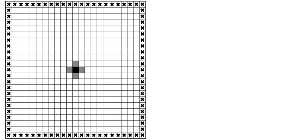
Figure 1. Simulation area and the boundary in PoissonLaplace equation systems. A black square located at the center of the domain expresses the only network cell in the initial stage, which functions as a seed of the network. Four gray squares surrounding a black square express the critical cells, which are the candidates possible to be a network cell in the second stage. In general, the cells located along the tree network “river” can be the next network cell. The boundary cells are represented by crosses (×), in which Dirichlet boundary conditions (u = 0 or u = 1) or Neumann boundary conditions (∂u/∂n = 0) are imposed, as shown in Table 1. The figure above is drawn in the domain with 23 × 23 cells, although the simulations in this article are carried out in the 43 × 43 domain. The network “river” never reaches the boundary, unless all the inside cells are included in the network (u = 0). Thus, the boundary is not drawn in the following simulation images, then, the total number of cells is 41 × 41 (=1681).

Table 1. Simulation settings in Poisson-Laplace equation systems.
Three kinds of settings are employed in simulations of Poisson-Laplace equation systems. When the selection rule is MAX, the cell with the maximum u-value is selected among the critical cells. Meanwhile, the cell with the minimum u-value is selected, when the selection rule is MIN. The “critical cell” means the candidate cell adjacent to the network, which is expected to be a new network cell in the next step. Further, the “network cell” means the cell that is already a component of the existing network (u = 0). As for f(x,y), the absolute values have no meaning, because the simulation systems in this article are conceptual models. In the case of the Poisson equation model, f(x,y) ≠ 0 is essential.
2.3. Selection Rules
At the starting point of simulations, t = 0, the number of the network cell is only one, which functions as a seed of the network. Assuming that the u-value of network cells is zero, the number of cells with u = 0 at the starting point is also one except for the boundary cells. Figure 1 is the case in which the initial network cell is located at the center of the domain, which is shown by the black square. There are four candidates adjacent to the black cell that can be the second network cell in the next step, t = 1, which are called “critical cells” and shown by the gray squares in Figure 1. Thereafter, one cell is chosen among the critical cells and changed into the network cell in each step. Thus, the number of the network cells continues to increase one by one in every step of the simulation. Figure 2 shows the distributions of the initial u-values corresponding to three settings, Sets I, II and III.
Two types of selection rules are employed on the choice of the next network cell among the critical cells, which are named “MAX” and “MIN”, respectively. In the case of MAX, the cell that has the largest u-value is selected, while in the case of MIN, the cell that has the smallest u-value is selected. It should be noted that a matter of importance is not the u-value itself but the gradient to the adjacent network cell. However, if the interval between cells h is constant, the u-value of a critical cell and its gradient are precisely proportional with each other, because u-values of the network cell are zero everywhere. All the u-values are determined by the Poisson or the Laplace equation, which is repeatedly calculated throughout the simulations. Thus, one of the critical cells lying by the existent network pattern is chosen and falls into the network step by step depending on whether the u-value of the corresponding cell is the largest or the smallest.
2.4. Finite Difference Method (FDM)
The mechanisms to simulate tree network formation by the Poisson or Laplace equations are well known. However, it is not so easy to design the practical PC programs, because a lot of memories and long elapsed time are required.
In Computer Aided Engineering (CAE), several methods such as the Finite Element Method (FEM), the Boundary Element Method (BEM) and the Finite Difference Method (FDM) are used to analyze mathematical models described by differential equations. In the simulations of this article, the simulation area is a square lattice, and it is easy to divide the area into small squares of the same size. In such cases as the shape of the boundary is not complicated, the best choice is the FDM, because the simulation speed of the FDM is much faster than those of the FEM and the BEM. Then, we adopt the improved FDM for the analyses of the Poisson-Laplace equation system in this article.
In any way, when solving a Poisson or a Laplace equation, we must deal with simultaneous linear equations with a great number of unknown variables. In the simulations of this article, the number of variables rises to 41 × 41 (=1681). However, the square matrix describing the simultaneous linear equations is symmetric. Then, the Cholesky method can be implemented, which saves a lot of time and relieves a lot of labor accompanied with simulations.
The procedures to apply the FDM are as follows. First, Equation (1) is discretized using the following formula.
 (2)
(2)
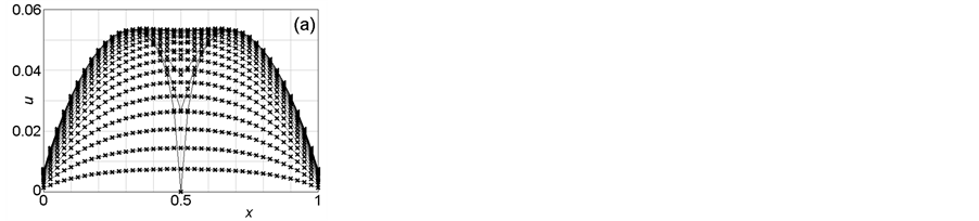
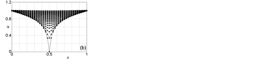
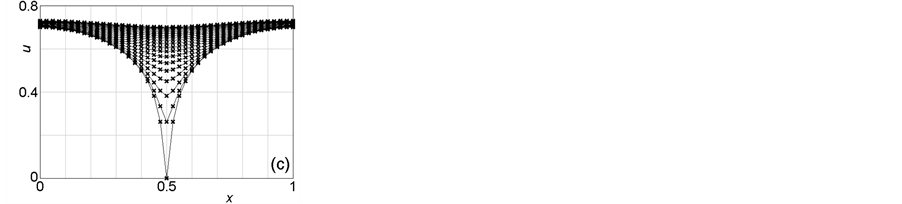
Figure 2. Profiles of u-values at the starting point of simulations. (a) Set I: Dirichlet boundary conditions (u = 0). (b) Set II: Dirichlet boundary conditions (u = 1). (c) Set III: Neumann boundary conditions (∂u/∂n = 0). For all settings, the u-value of the central cell is zero at the starting point of simulations. The abscissa stands for the central position of each cell along the x-axis, which varies from 0 to 1. The interval between adjacent cells h = 1/N (N = 40).
As a result, Equation (1) is deformed, such as
 (3)
(3)
 (4)
(4)
Next, a total of (N + 1) × (N + 1) cells constituting the simulation area are consecutively numbered in order from the lower left to the upper right, that is, from n = 0 to N × (N + 2). Using the signs “%” and “/” to represent the remainder and the quotient, respectively, the relations between the coordinates nx, ny and the consecutive number n are as follows.
 (5)
(5)
Then, Equation (4) is rewritten using arrays, such as
 (6)
(6)
Here, the variable n is varied from 0 to N × (N + 2). Signifying u[n] and f[n] as un and fn, respectively, we can reach the following simultaneous linear equations, consisting of (N + 1) × (N + 1) equations.
 (7)
(7)
For each setting, i.e., Set I, II or III, the simultaneous Equations (7) are solved by the FDM. The values of the matrix elements Aij differ slightly with each other corresponding to the settings.
In the case that a seed of the network is located at the center of the domain in the initial stage, whose u-value is zero, uN(N+2)/2 = 0, the values of the following matrix elements in the left side and an f-value in the right side are changed, such as
 (8)
(8)
Figure 2 shows the initial distributions of the u-values at this time corresponding to Sets I, II and III, respectively.
In every step, the whole u-values are recalculated using the FDM and redistributed on the simulation area. Then, one of the critical cells adjacent to the current network is chosen and changed into the new network cell according to the selection rule MAX or MIN. For example, when the n-th cell is a new network cell, i.e., un = 0, the values of following matrix elements and fn are changed, as follows.
 (9)
(9)
These constitute a new boundary condition. Then, the next calculation and distribution restart. Thereafter, this process is repeated, and the cells whose u-value is zero continue to increase one by one as the simulation succeeds. In this way, the tree network pattern is renewed and gradually developed.
3. Simulation Results
3.1. Temporal Evolution of Poisson-Laplace Equation Systems
Figure 3 shows the temporal variation of simulation patterns in Set I, where the Poisson equation model and the MAX selection rule are employed. That is, the cell with the maximum u-value is chosen as a next network cell. A gradual development of the tree-shaped network structure is observed. On the other hand, Figure 4 is the temporal variation in Set II, where the Laplace equation model and the MIN selection rule are used. When the cell with the minimum u-value is chosen, the disk-like filled pattern is formed in the central area, and no tree network structure is developed. Distinct contrast in Figure 3 and Figure 4 is the main theme of this article, which is later discussed in Section 4.1 in detail.
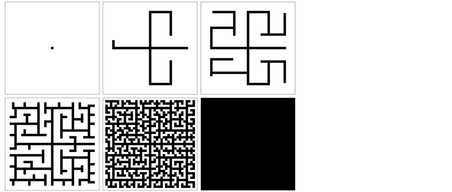
Figure 3. Temporal evolution of the Poisson equation model (Set I). The simulation area without the boundary is composed of 41 × 41 (=1681) cells. From the upper left to the lower right, the patterns are those at t = 0, t = 105, t = 210, t = 420, t = 840 and t = 1680, respectively. As one cell falls into the network at every unit time, the total numbers of network cells are n = 1, n = 106, n = 211, n = 421, n = 841 and n = 1681, respectively. In the case of Set I, the tree network structure is gradually developed with the increase in time. Once one of symmetric cells is chosen, any symmetry begins to be lost. The final state, where all cells are included within the network, could indicate the ultimate equilibrium in correspondence with “heat death” in the universe.
Figure 4. Temporal evolution of the Laplace equation model (Set II). From the upper left to the lower right, the patterns are those at t = 0, t = 105, t = 210, t = 420, t = 840 and t = 1680, respectively. In the case of Set II, the tree network structure is not developed. The fact that the final states are the same both in Figure 3 and Figure 4 suggests that the ultimate equilibrium is inevitable for all systems whether the intermediate state is dissipative or not.
The temporal variations of the critical and the average u-values in Sets I and II are examined in Figure 5 and Figure 6, which correspond to Figure 3 and Figure 4, respectively. Here, the term “critical” means “just chosen as an additional plus-one network cell in the latest step” according to the selection rule MAX or MIN. Meanwhile, the average u-values are calculated for all inner cells, the number of which is 41 × 41 (=1681). Comparison between Figure 5(b) and Figure 6(b) clarify that the decreasing rate of the average u-value in the Set I simulation is larger than that in the Set II simulation, which reflects the difference between the MAX and MIN selection rules.
3.2. Simulations of River Channel Formation
In comparison between Figure 3 and Figure 4, it appears that network formation necessitates the Poisson equation model and the MAX selection rule. On the basis of this observation, we apply the Poisson equation model of Set I to simulations of natural phenomena such as river channel formation [2] [13] [17] -[19] . At this time, the introduction of random functions is inevitable in order to get more natural and realistic images.
The simulations of river channel formation are conducted in the same square area as those in Figure 3 and Figure 4. Then, one of the cells is chosen as the outlet or drain in the initial state. It is assumed that the u-values of the network cell, which is the component of river channels, are all zero, meaning that water can flow freely throughout the channels.
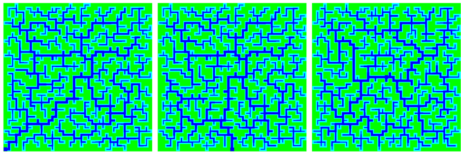
The simulation results are shown in Figure 7 for three different outlet positions using the same random number table. The outlets are placed at the lower left corner (a), the center of the lower side (b) and the center of the domain (c), respectively, which are shown by comparatively large squares. The random numbers are varied from 0.5 to 1.5, and the calculated u-values are divided by these numbers. Thus, it becomes that the u-values are randomized within the range between 2/3u and 2u. It should be noted that the u-values are not multiplied but divided by random numbers, the reason of which is explained in Section 4.3. Each simulation continues until more than half of the inner cells are changed into the network cell, that is, the component of the water channel.
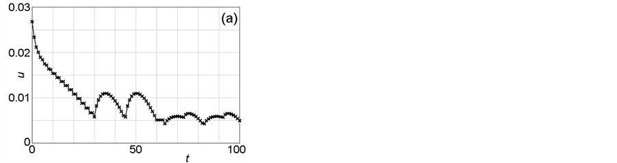
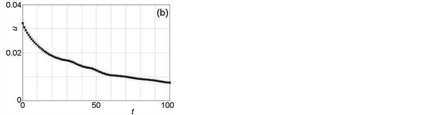
Figure 5. Temporal variations of critical (a) and average (b) u-values (Set I). These figures correspond to Figure 3. The “critical u-value” means the u-value of the cell just changed to the network cell in the latest step. The average u-value is calculated for all 41 × 41 (=1681) cells within the simulation area. At every unit time, one block falls into the network. Figure 5(b) shows that the total flow resistance is monotonically decreased with time passing.
Figure 6. Temporal variations of critical (a) and average (b) u-values (Set II). These figures correspond to Figure 4. It should be noted that the monotonic decay in the total flow resistance in Figure 6(b) is slower than that in Figure 5(b).
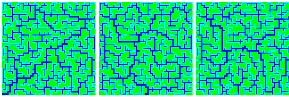
One more simulation setting, Set III, is newly introduced, and the simulation results are shown in Figure 8, where the Poisson equation model and the selection rule MAX are employed as well as Set I. However, the Dirichlet boundary condition is altered to the Neumann boundary condition, where ∂u/∂n = 0, meaning that the u-values of the boundary cells are the same as those of the nearest inner cells. Despite slightly different images are obtained, we can say that any essential differences are not recognized compared with the images in Figure 7. The same random number table is used as in Figure 7.
4. Discussion
4.1. Necessary Conditions for Tree Network Formation
First of all, we stress that the Poisson and the Laplace equation models adopted in this article are conceptual models. There is no meaning in the absolute values of the two-dimensional functions u(x,y) and f(x,y). Of importance are only relative values. Although f(x,y) = 1 in the Poisson equation models, we can get the same simulation results for any positive values of f(x,y).
In this article, we deal with three simulation settings, Sets I, II and III, because these settings satisfy the most fundamental condition that some kinds of meaningful (not trivial) patterns are formed within the simulation area, whether it is a tree network or not. For example, suppose the Laplace equation model in which the Dirichlet
 (a) (b) (c)
Figure 7. Tree network formation in river channel simulations (Set I). The outlets from which water is discharged are located at the lower left corner (a), the center of the lower side (b) and the center of the domain (c), respectively, which are illustrated by comparatively large squares. The random function is introduced in order to get more natural and realistic images, where the u-values are randomized within the range between 2/3u and 2u. In Figure 7 and Figure 8, simulations are completed when the total number of the network cell exceeds the half (841 cells). The later, the thinner line is drawn.
 (a) (b) (c)
Figure 8. Tree network formation in river channel simulations (Set III). Dirichlet boundary conditions (u = 0) are replaced by Neumann boundary conditions (∂u/∂n = 0) for these simulations. The same random number table is used as in Figure 7.
boundary condition and the MAX selection rule are employed. Then, if the u-values of the boundary u = 0, any pattern formation does not progress. If u = 1, any pattern is not formed in the central area, because the pattern goes straight toward the boundary and roams around there. In these cases, we judge that the system is diverged and that any meaningful pattern formation cannot be performed. That is, such settings are excluded in the numerical simulations of this study from the beginning.
As shown in Section 3, tree network formation succeeds when Sets I and III are chosen. On the other hand, when the simulation setting is Set II, tree network formation fails. Common characteristics in Sets I and III are the following two: the Poisson equation with the finite value of f(x,y) and the MAX selection rule. On the contrary, both conditions are lacking in Set II. Thus, it is concluded that these two, the Poisson equation and the MAX selection rule, are necessary conditions for tree network formation.
4.2. Tree Network Formation and the MEP Principle
It is supposed that the first condition, the Poisson equation, guarantees the exchange of energy and materials with external environment, because the finite value of f(x,y) characterizes the existence of divergence, which means the input and the output of energy and materials. This condition also guarantees the state far from equilibrium, which can advance the formation of dissipative structures. Meanwhile, the Laplace equation with f(x,y) = 0 does not guarantee the exchange with external environment, meaning that the system lies in the isolated state or the state near equilibrium at the best.
It is clear that the second condition, the MAX selection rule, substantiates the Maximum Entropy Production (MEP) principle, because the u-values are directly proportional to entropy. When the critical cell with the maximal u-value is changed into the network cell, the u-value of which is zero, it is clear that the maximal entropy is produced and emitted to the external environment.
Different from the view of Kleidon et al. [7] , we cannot confirm the influences of boundary conditions in the numerical experiments of this article. For example, tree network formation is advanced even in Set I, despite the Dirichlet boundary conditions are employed, where the u-values of the boundary are fixed and unchangeable. Considering that most simulations in this study are ended until the network cells occupy a half of the simulation area, disagreement is probably because the influences of boundary conditions are not so outstanding until the middle stage of simulations.
Assume an extreme case where the simulation is continued to the end as in Figure 3 and Figure 4. It is easy to surmise that no difference is found in simulation results of three settings, Sets I, II and III. Exactly the same image must be seen for three settings, where all cells are changed into the network cell, and the simulation area is filled by the cells with u = 0. Any pattern has been washed away. It is suggestive that these images correspond to final equilibrium, “heat death”, which is unavoidable for any existence in the universe. The final winner is always the “thermodynamic equilibrium”.
The main theme of this study is to present the mathematical model that can certify the effect of the MEP principle. The correlations between the model setting and the created pattern discussed in this section are summarized in Table 2.
So far, the MEP principle is still no better than a hypothesis. It is not yet mathematically proved. There are many scientists who do not support the MEP principle. We expect that the Poisson equation model constructed in this article exemplifies the MEP principle in the simulation world.
4.3. Consistency with the Constructal Theory
The constructal theory by Bejan et al. insists that the flow system such as area-to-point flow is optimized in such a way that the global flow resistance is minimal and that the flow configuration provides easier access to the
Table 2. Correlations between simulation settings and created patterns.
MEP and MinEP are the abbreviations of Maximum Entropy Production and Minimum Entropy Production, respectively.
current flow [12] [13] . It is obvious that the Poisson-Laplace equation system in this article is a typical example of area-to-point flow. The simulation results of both the Poisson and the Laplace equation models show the overall decrease in u-values, as shown in Figure 5 and Figure 6. This observation seems to be consistent with the prediction of the constructal theory, suggesting that the geometrical structure in the Poisson-Laplace equation system is also stabilized so that the total flow resistance is minimal.
However, these results are not surprising, taking account of the simulation method where non-network cells with positive u-values continue to be transformed into the network cells with zero u-values. Here, of great importance is the decreasing rate of the u-value, i.e., the decreasing speed. As shown in the simulation results of Figure 5(b) and Figure 6(b), the decreasing speed in Set I is much faster than that in Set II. This observation strongly supports the MEP principle, where the decreasing speed of total entropy should be maximal in order to promote the formation of dissipative structures.
4.4. Origin of Randomness in River Channel Formation
As shown in Figure 7 and Figure 8, we can get more natural and realistic images by using random number tables. If so, what is the basis to introduce random numbers in river channel formation? In these simulations, the output u-values are divided by random numbers before compared with each other. Why are these u-values divided by random numbers instead of multiplied?
As discussed in Section 4.1, the MAX selection rule is indispensable for tree network formation. According to the MAX selection rule, the cell whose u-value is the largest is chosen and changed into the network cell. Strictly speaking, the rule should be corrected as follows: the cell whose gradient is the largest is chosen and changed into the network cell. Thus, the values that should be compared are not u-values. Considering that the u-values of network cells are all zero, the gradients are calculated by dividing the u-values by h, where the denominator h represents the interval between the corresponding cell and the nearest network cell. If all the intervals are equal, it is allowed to compare directly with u-values, because u-values and gradients are exactly proportional with each other.
However, when the simulation area is disturbed and the intervals between the cells are not equal depending on the site, the situation is different. If it can be assumed that the disturbances of the simulation area are caused by natural factors such as unevenness of topography, it is reasonable to randomize the interval h. This is the reason why comparison is not carried out between u-values but between those divided by random numbers.
It is not so easy to fully incorporate the effects of disturbances into simulation processes. For example, when the simultaneous linear equations are solved to get u-values, it is assumed that the interval h is constant, and disturbances are not taken into account. Thus, the choice of division or multiplication might not influence simulation results significantly.
4.5. MEP Principle and the Second Law of Thermodynamics
The MEP principle states that physical or biological systems continuously exchanging a large quantity of energy and materials with the external environment maintain steady states in which entropy production is maximized. Other preconditions are a sufficient degree of freedom, unfixed boundary conditions, etc. Meanwhile, it is also known that dissipative structures stabilized in the state far from equilibrium are characterized by low entropy. It seems that these two statements are inconsistent with each other. How can we compromise the contradiction? At the end of this article, we would like to refer to this issue.
The dilemma could be solved by dividing the system into two parts, the inside and the outside of the system, that is, the internal dissipative structure and the external environment [7] . In Figure 9, two areas are drawn by the dark gray color and the light gray color, respectively. It should be noted that energy, heat and materials continue to flow within the whole system. There exists a steep gradient in energy and materials from the source to the sink, which can induce a large scale of diffusion. For example, the heat source of the Earth system is the Sun and the heat sink is the outer space. Consequently, two streams are generated in the whole system, one of which diffuses directly within the external environment, i.e., the outer space, and the other of which passes through the dissipative structure, i.e., the Earth system. These streams are shown by the black arrows in Figure 9(a).
With Sint and Sext being entropy generated in the dissipative structure and in the external environment, respectively, total entropy Stot in the system is represented by the sum of Sint and Sext, as follows.
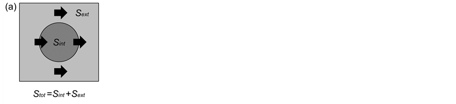
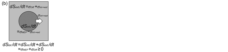
Figure 9. MEP principle and the second law of thermodynamics. The internal dissipative structure and the external environment are expressed by the central dark gray circle and the surrounding light gray area, respectively. (a) The black arrows show the fluxes of energy and materials, which are divided into two flows, the flow via the dissipative structure that give rise to the state far from equilibrium and that of direct diffusion within the external environment. Total entropy in the whole system Stot is represented by the sum of entropy in the internal dissipative structure Sint and that in the external environment Sext, i.e., Stot = Sint + Sext. (b) The entropy production rate in the whole system dStot/dt is represented by the sum of the rate in the dissipative structure dSint/dt and that in the external environment dSext/dt, i.e., dStot/dt = dSint/dt + dSext/dt. The entropy production rate within the dissipative structure is represented by the difference between the entropy production rate by the MEP principle σMEP and that from the internal system to the external environment σint®ext, which is shown by the white arrow. Entropy production by direct diffusion σDiff also takes place within the external environment. Thus, entropy production in two regions can be described by dSint/dt = σMEP – σint®ext and dSext/dt = σDiff + σint®ext, respectively. If the whole system can be regarded as isolated, the second law of thermodynamics should hold, which is guaranteed as dStot/dt = σMEP + σDiff ≥ 0. When the internal system is in the steady state, dSint/dt = 0, thus, σMEP = σint®ext.
 (10)
(10)
Moreover, the differentiation of Equation (10) leads to the following equation.
 (11)
(11)
Two kinds of entropy production can arise due to above mentioned streams. These are entropy production by direct diffusion σDiff and that by the MEP principle σMEP, which occur within the external environment and the internal system, respectively. Beside these two, the entropy flow from the internal to the external system also exists, whose rate is signified by σint®ext. Thus, entropy production rates within the internal system dSint/dt and the external environment dSext/dt are described, respectively, as follows.
 (12)
(12)
Entropy production in these processes is shown in Figure 9(b). The white arrow expresses the entropy flow from the inside to the outside σint®ext.
Assuming that the external environment contains energy sources such as the Sun, the whole system could be considered almost isolated. Consequently, the second law of thermodynamics should hold, which is confirmed, as follows.
 (13)
(13)
Taking into consideration that the spatial area of dissipative structures such as the Earth occupies only a small part of the whole system such as the heliosphere, the amount of σDiff should be much larger than that of σMEP.
If the internal system exists in the steady state, entropy production in this region can be annihilated, i.e., dSint/dt = 0, which leads to the following relation.
 (14)
(14)
Then, we can propose the following interpretations as for the MEP principle.
1) Entropy production during the formation of the dissipative structure is maximized.
2) When the dissipative structure is in the steady state, that is, the total entropy production rate within the dissipative structure is zero, entropy generated in the process 1) is wholly transmitted from the dissipative structure to the external environment.
3) As a result, the residual entropy amount in the dissipative structure is minimized, which guarantees low entropy in the internal dissipative structure.
According to the interpretation above, dissipative structures can maintain a state of low entropy by “discarding” high entropy fluxes out of the system [7] . Our Poisson-Laplace equation system presented here will strongly back these interpretations.
5. Conclusions
1) The Poisson equation model assisted by the FDM is an effective and practical tool to simulate tree-shaped network patterns, which are frequently observed in natural phenomena such as river channel formation.
2) The Poisson equation model designed to simulate the state far from equilibrium and to satisfy the MEP principle can create fractal tree network patterns. Meanwhile, the Laplace equation model designed to simulate the state near equilibrium and to satisfy the MinEP principle cannot. The Poisson-Laplace equation system constructed in this study can be a conceptual simulation model that testifies the effect and the validity of the MEP principle.
3) In the system exchanging abundant energy and materials between the dissipative structure and the external environment, entropy is radiated from the inside to the outside of the system, i.e., from the internal dissipative structure to the external environment. At this time, entropy radiation is maximized in accordance with the MEP principle. Low entropy of dissipative structures is guaranteed by disposing a large scale of entropy to the external environment. However, entropy in the whole system including both the dissipative structure and the external environment increases in time, which reconciles the controversy between the MEP theory and the second law of thermodynamics.
Acknowledgements
This study is partly supported by the Global COE program “Global Eco-Risk Management from Asian Viewpoints” and by Grant-in-Aid Project DDT01304.
References
- Mandelbrot, B.B. (1982) The Fractal Geometry of Nature. Freeman, San Francisco.
- Rodriguez-Iturbe I. and Rinaldo, A. (1997) Fractal River Basins: Chance and Self-Organization. Cambridge University Press, Cambridge.
- Shimokawa M. and Ohta, S. (2012) Annihilative Fractals Formed in Rayleigh-Taylor instability. Fractals, 20, 97-104. http://dx.doi.org/10.1142/S0218348X12500090
- Prigogine, I. (1962) Introduction to Non-Equilibrium Thermodynamics. Wiley-Interscience, New York.
- Prigogine, I. and Stengers, I. (1984) Order out of Chaos: Man’s New Dialogue with Nature. Bantam Books, New York.
- Kondepudi D. and Prigogine, I. (1998) Modern Thermodynamics: From Heat Engines to Dissipative Structures. John Wiley & Sons, New York.
- Kleidon A. and Lorenz, R.D. (2004) Entropy Production by Earth System Processes. In: Kleidon, A. and Lorenz, R.D., Eds., Non-Equilibrium Thermodynamics and the Production of Entropy: Life, Earth, and Beyond, Springer-Verlag, Berlin, 1-20.
- Martyushev L.M. and Seleznev, V.D. (2006) Maximum Entropy Production Principle in Physics, Chemistry and Biology. Physics Reports, 426, 1-45. http://dx.doi.org/10.1016/j.physrep.2005.12.001
- Schrödinger, E. (1944) What Is Life? The Physical Aspect of the Living Cell. Cambridge University Press, Cambridge.
- Shimokawa S. and Ozawa, H. (2002) On the Thermodynamics of the Oceanic General Circulation: Irreversible Transition to a State with Higher Rate of Entropy Production. Quarterly Journal of the Royal Meteorological Society, 128, 2115-2128. http://dx.doi.org/10.1256/003590002320603566
- Meysman F.J.R. and Bruers, S. (2010) Ecosystem Functioning and Maximum Entropy Production: A Quantitative Test of Hypotheses. Philosophical Transactions of the Royal Society B-Biological Science, 365, 1405-1416. http://dx.doi.org/10.1098/rstb.2009.0300
- Bejan A. and Lorente, S. (2006) Constructal Theory of Generation of Configuration in Nature and Engineering. Journal of Applied Physics, 100, Article ID: 041301. http://dx.doi.org/10.1063/1.2221896
- Bejan, A. (2007) Constructal Theory of Pattern Formation. Hydrology and Earth System Sciences, 11, 753-768. http://dx.doi.org/10.5194/hess-11-753-2007
- Kleidon, A. (2010) Life, Hierarchy, and the Thermodynamic Machinery of Planet Earth. Physics of Life Reviews, 7, 424-460. http://dx.doi.org/10.1016/j.plrev.2010.10.002
- Bejan, A. (2010) Design in Nature, Thermodynamics, and the Constructal Law. Comment on “Life, Hierarchy, and the Thermodynamic Machinery of Planet Earth” by Kleidon. Physics of Life Reviews, 7, 467-470. http://dx.doi.org/10.1016/j.plrev.2010.10.008
- Kleidon, A. (2010) Life as the Major Driver of Planetary Geochemical Disequilibrium. Reply to Comments on “Life, Hierarchy, and the Thermodynamic Machinery of Planet Earth”. Physics of Life Reviews, 7, 473-476. http://dx.doi.org/10.1016/j.plrev.2010.11.001
- Errera M.R. and Bejan, A. (1998) Deterministic Tree Networks for River Drainage Basins. Fractals, 6, 245-261. http://dx.doi.org/10.1142/S0218348X98000298
- Marin C.A. and Errera, M.R. (2009) A Comparison between Random and Deterministic Dynamics of River Drainage Basins Formation. Engenharia Térmica (Thermal Engineering), 8, 65-71.
NOTES

*Corresponding author.