Natural Science
Vol.5 No.3(2013), Article ID:29032,7 pages DOI:10.4236/ns.2013.53050
Lattice Boltzmann modeling for tracer test analysis in a fractured Gneiss aquifer
![]()
1TU Bergakademie Freiberg, Instuite for Geology, Freiberg, Germany; ramawaad@gmail.com, merkel@geo.tu-freiberg.de
2Florida International University, University Park, USA; andrew.j.pearson@gmail.com
Received 4 January 2013; revised 6 February 2013; accepted 21 February 2013
Keywords: LBM; QTRACER2
ABSTRACT
Fractured Gneiss aquifers present a challenge to hydrogeologists because of their geological complexity. Interpretation methods which can be applied to porous media cannot be applied to fractured Gneiss aquifers because flow and transport occur in fractures, joints, and conduits. In contrast, the rock matrix contribution to groundwater flow is not very important in Gneiss aquifers. Sodium chloride was injected into groundwater flow under steady state condition as tracer to determine transport parameters which are needed for transport modeling. QTRACER2 was used to evaluate the tracer test data. Lattice Boltzmann method was applied to simulate flow and tracer transport through a fracture zone in Gneiss. Experimental tracer data and the numerical solution by lattice Boltzmann method are compared. In general, the results indicate that a 2D Lattice Boltzmann model is able to simulate solute transport in fractured gneiss aquifer at field scale level.
1. INTRODUCTION
A major difficulty modeling fractured aquifers is the high degree of uncertainty in aquifer geometry, specifically fracture geometry, distribution and fracture aperture. Solute transport in fractured aquifers is important for environmental aspects and poses additional problems by matrix diffusion within the fracture zone due to fracture filling sediments.
Tracer tests are favourable to estimate aquifer geometry and transport properties. They may be executed in laboratory experiments or small and regional scales. Many efforts have been made to test tracer transport in fractured aquifers [1-4]. Tracers are defined as chemical substances which may be inorganic and organic constituents in water, isotopes or very small particles. The tracer may be present due to environmental processes or introduced by man into the aquatic environment [5]. Tracer tests are commonly used in fractured aquifers to provide a better overview about the connectivity of fractured aquifer.
Tracer test can be classified into the following groups: conservative, partitioning, and other tracer tests. The conservative tracer remains in a single phase (e.g. water) while partitioning tracer partition into another phase (e.g. gas). Tracer tests can be conducted in steady state or transient mode. Injection of one or more tracers at a time is possible [6-11]. Interpretation of tracer test can be numerical and analytical, but the analytical analysis is restricted to steady state flow while numerical analysis can deal with steady or transient state flow.
Pumping tests with packers and geophysical borehole investigations were used to identify the hydraulic properties and important fractured zones in the Gneiss aquifer of Freiberg. It was found that the uppermost horizontal fracture is the most important zone within the hydrogeological test site of the TU Bergakademie Freiberg [12].
Several analytical and numerical solutions have been developed during the last decades to simulate flow and solute transport in porous and fractured aquifers. A widely used approach in surface water and groundwater environments is the Advection-Dispersion Equation (ADE) with three mechanisms controlling solute transport: advection, dispersion, and diffusion. Hydrodynamic dispersion was first observed by Slichter [13]. Bear [14] classified three methods to simulate the flow in fractured flow. The methods are Equivalent Porous Medium method (EPM), Double Porosity Method (DP), and Stochatsic Discrete Fracture Network method. However, several dual-permeability models have been developed to describe the flow and solute transport in the fractured aquifer [e.g. [15-17]]. Solute advection and dispersion take place in both pore systems. Applying stochastic method to study groundwater flow and contaminant transport in dual porosity media with random hydraulic conductivity is relatively limited. For example, Hu et al. [18] developed a stochastic Eulerian perturbation approach for stochastic analysis of solute transport in heterogeneous, dual-permeability media.
Lattice Boltzmann modeling (LBM) is a rather new numerical technique for complex fluid flow where Darcy’s law can not been applied. Instead of solving the Navier-Stokes equations describing the flow of a Newton fluid, the discrete Boltzmann equation describes flow of a Newton fluid by using a limited number of particles. LBM was built initially to deal with fluid flow described by the Navier-Stokes equations [19-21]. Flekkøy [22] addressed low diffusion in LBM and confirmed that the diffusion coefficient is obtained by the relaxation value. Gutfraind et al. [23] used lattice gas (a forerunner of LBM) to study the relation between fracture aperture and hydrodynamic dispersion. Yeo [24] investigated the effect of fracture roughness and fluid velocity with different geometry (amplitude and wavelength) on solute transport using LBM. He et al. [25] compared between the lattice Boltzmann method and an isothermal NavierStokes method. Yoshino and Inamuro [26] computed the species transport in porous media by using 3D LBM. Zhang and Ren [27] explored different boundary condition for one dimension vertical leaching LBM.
Lattice Boltzmann model (LBM) is a powerful tool not only for simulating fluid flow but as well solute transport in porous media and fractured aquifers [28,29]. Today, many different lattice Boltzmann models exist. A popular approach for 2D simulation is D2Q9 (Figure 1),

Figure 1. Shows D2Q9 model (modified after Sukop, 2006).
while for 3D simulation D3Q15, D3Q19, and D3Q27 are commonly used. Dn denotes for the number of dimensions and Qn denotes for number of velocities per lattice site (e.g. D2Q9 is a two dimensional Lattice Boltzmann model with nine velocities).
Figure 1 shows the Cartesian lattice with 9 velocity and directions of a D2Q9 model. Point 9 represents the particle at rest (zero velocity).
QTRACER2 was designed to be used for Karst systems primarily, but it handles fractured aquifer as well [30]. It is widely used to evaluate tracer tests in surface water, porous media, Karst, and fractured aquifers. Tam [31] estimated e.g. the mean tracer transit time and conduit volume between a sinkhole and resurgence by QTRACER2. Birk et al. [32] interpolated tracer test results for a carbonate system using three different methods, namely the method of moment, Analytical Advection Dispersion models (ADMS), and numerical solution. Massei et al. [33] calculated hydrodynamic and transport parameters for a Karst-conduit system with QTRACER2 using linear graphical (method of moments) and Chatwin methods. GABROVŠEK [34] determined the dispersion coefficient using the Chatwin method in QTRACER2 for an impulse tracer test.
2. THEORY
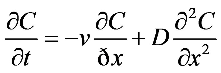
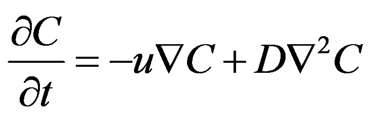
Bear [35] wrote Advection-Dispersion equation (ADM) for solute transport in porous media as follows:
 . (1)
. (1)
Here, C is the solute concentration, v the advection velocity and D the dispersion coefficient. The method of moment in QTRACER2 is based on the analytical solution of the following one-dimensional advective-dispersion Eq.2:
 (2)
(2)
with (3)
(3)
C(t) is the concentration at a time (t), (m) is the quantity of injected mass, (X) is the distance between the injection and observing point, (Qm) is the flow rate, (DL)is the longitudinal dispersion, (P) is the Peclet number, and tm is the mean transit time.
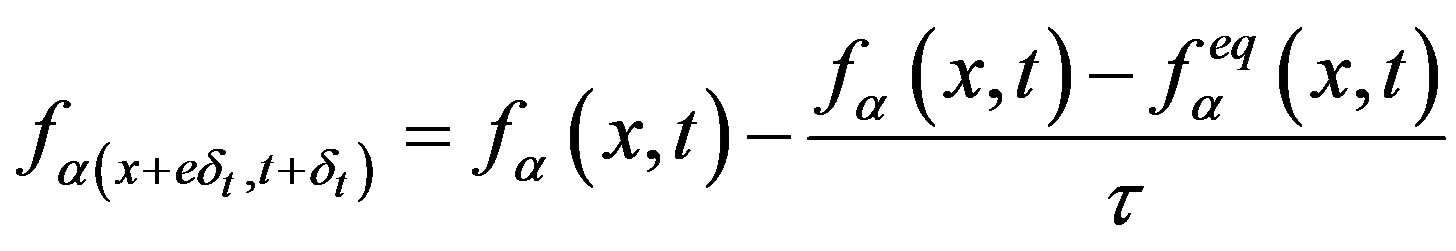
LBM can be driven from the continuous Boltzmann equation [36] and given by:
 . (4)
. (4)
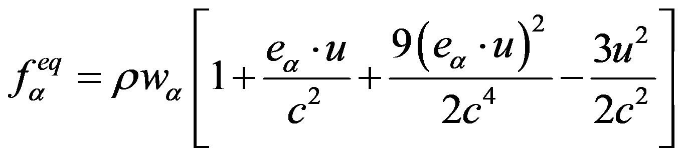
The right side of the equation is the collision operator with α representing one of the principal directions and  representing the equilibrium distribution function [37] which is given by:
 . (5)
. (5)
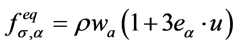
cs (1/√3lu ts−1) is the sound speed, u is the macroscopic velocity and τ is the relaxation time which calculates the viscosity. However, each component fluid and solute has a specific. Because the solute will be move as passive scalars, the truncated equilibrium distribution function for solute transport [37] is given by:
 . (6)
. (6)
σ depicts the solute transport component and velocity is attained from the fluid flow. Thus, the solution of the advection-diffusion equation is:
 . (7)
. (7)
C denotes the solute concentration, t time, and D is the diffusion coefficient.
3. TRACER TEST AND SETUP
No tracer tests have been done so far to estimate the transport properties in the Freiberg Gneiss fractured aquifer. Around the world, only a few tracer tests were conducted in Gneiss aquifers [38]. In fact, there is no ideal tracer appropriate for all sites. However, there is always an optimum tracer for the site but the tracer fits of the area cannot be suitable for another area.
A natural gradient tracer test was applied, where a tracer injected into the groundwater water move under prevailing natural condition. This approach had advantages and disadvantages. An advantage of this approach is that it is representative of natural conditions. One disadvantage is the rather long time required for monitoring and sampling [39].
In this experiment, a salt solution (NaCl) was injected into well no 4 (Figure 2) in early October of 2011 at the well field of TU Bergakademie Freiberg. A tracer solution was mixed using 1 kg sodium chloride and 100 Liter water. The water was heated to compensate the density difference and concentration was rather low to avoid problems with density difference. The injected time was 6.5 hours.
Sodium chloride is inexpensive, easy to use, easily detectable by reading the electrical conductivity, and environmental friendly. The EC was read every 10 minutes by CTD Divers, which were installed in the wells a few days before the injection. The tracer test can be divided into two phases: the injection phase and the monitoring phase. Figure 2 illustrates the initial groundwater level and well locations in the experimental area.
Two pneumatic packers were used in well no 4 to isolate the major fracture zone at a depth of 11 to 12 m below surface. The injection started on October 9, 2011 with a constant rate of 260 ml/min for a period of 6.5 hours. Electric conductivity was measured in all monitoring wells over time with CTD divers reading pressure, electric conductivity, and temperature.
4. EVALUATION OF TRACER TEST
QTRACER 2 [40] was used to interpret the breakthrough curve. The shapes of the breakthrough curve play an important role in calculating the hydraulic and transport properties of the system. Transport parameters like mean residence time, mean velocity, etc. were calculated by the method of moments which involves calculating the area under the breakthrough curve. The first moments method determines as well the mean residence time, and mean velocity while the second moments determines the longitudinal dispersion coefficient [41].

Figure 2. Initial groundwater level and well locations in study area.
5. MODELING TRACER TEST BY MEANS OF LBM
For the simulation a multi-component model was applied. The first component was the fluid and the second component was a passive scalar. This component behaves as a passive component having no velocity and is advected by the background fluid [29,37,42,43]. LBM was used in the interpretation of the monitoring data from the natural gradient tracer test. Because the transport of the tracer through the gneiss fracture rock is primarily through fractures diffusion into rock matrix is very small and considered as being negligible compared to fracture flow. Flow paths are assumed to carry the fluid flow and the solute transport. The tracer test was simulated with LBM by using LBSim software [44,45].
One of the most important things in LBM models are units because physical units have to be converted to LBM units to obtain relaxation parameters which are playing important role in LBM. Reynolds number (Re) and Schmidt number (Sc) were used to convert physical unit to lattice unit because both of them are non-dimensional values [29]. The relaxation parameters for fluids (τ0, τ1) must be larger than 0.5 to insure positive viscosity. For stability, the fluid velocity in LBM should be less than ~0.1 - 0.2. The model domain measures 800 lattice unit (lu) in X direction and 120 lattice unit in Y-direction. The boundary conditions for the solute are fixed flux inlet and zero gradient outlet. Initial condition was a zero concentration in the entire area of modeling. The Figure 3 depicts the model geometry and boundary condition (parameter distribution).
6. RESULTS AND DISCUSSION
The only significant readings and a breakthrough curve were obtained at well no 6. Figure 4 shows the observed salt concentration over time. The tracer was first detected after 7.83 hours. The distance between the injection and well no 6 is around 4.9 m. The highest tracer concentration recorded was 107 mg/L. Table 1 displays a calculated parameter for the salt tracer test after interpolation by QTRACER2.
The breakthrough curve is characterized as skewed to

Figure 3. Shows model domain and boundary condition and boundary condition. Properties were chosen by random distribution.

Figure 4. Observed salt concentration at monitoring well 6 started on 9 October 2011.
the right with a rapid rise to peak and a long tailing to the right. The long tail explains the exchange between mobile (Fracture or conduit) and immobile water in fine pores of fracture filling sediments (fracture matrix) zones. The arrival of the tracer in the observation well no 6 proves that the injection and observation wells are directly connected. The groundwater flow is in the direction of well no 6. High drawdown observed in Well no. 6 from the double packer test done before the tracer test support this [12].
Time for first arrival indicates the time needed for a tracer to arrive at the observation well. The shape of breakthrough curve is positively skewed, hence the peak time lie behind the mean tracer transit time. The concentration versus time in the Figure 4 shows a peak describing the max velocity.
Also, the figure shows a tailing which can be explained by diffusion from the gneiss fracture matrix. The
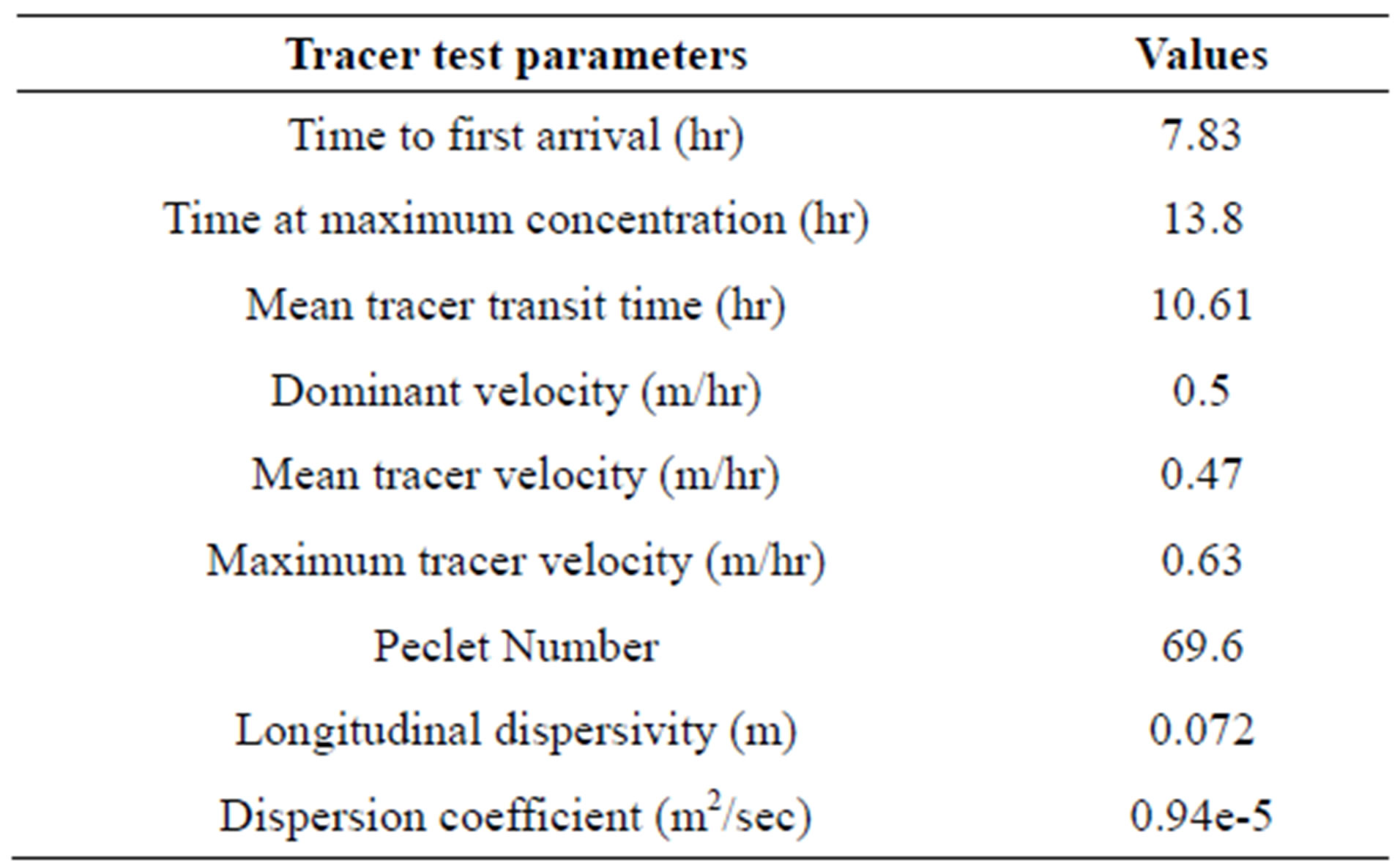
Table 1. Results from tracer test by QTRACER2 program.
concentration remained elevated for 180 hr before it returned to background level. The mean tracer transit time, dispersivity, dispersion, Peclet number, etc. are also found in Table 1. The Peclet number indicates advection control because the Peclet number is higher than 6 [46]. High Peclet number and small dispersion coefficient indicate a rather small degree of back-mixing. In other words, variance near zero meaning there is no back mixing.
LBSim software was run by using the calculated values from QTRACER2. To illustrate the efficiency of LBM to predict the BTC, the simulated dimensionless BTC compared to measured one are plotted in Figure 5. Figure 5 depicts the measured concentration versus time and calculated concentration versus time using LBM. It can be noted that observations fit rather well with calculated values.
Differences are more expressed in the tailing section of the BTC. It can be speculated that this is due to dead end pores and retention of the tracer in fracture matrix sediments.
7. CONCLUSIONS
QTRACER2 software allows rapid computation of transport parameters from the breakthrough curve. Method of moments within QTRACER2 provides handy tools to evaluate breakthrough curves. A rather good agreement between monitored and numerical breakthrough curves was found. Generally, Lattice Boltzmann showed a good simulation for the breakthrough curve but for long tail tracer test there is still a difference between measured and calculated values.
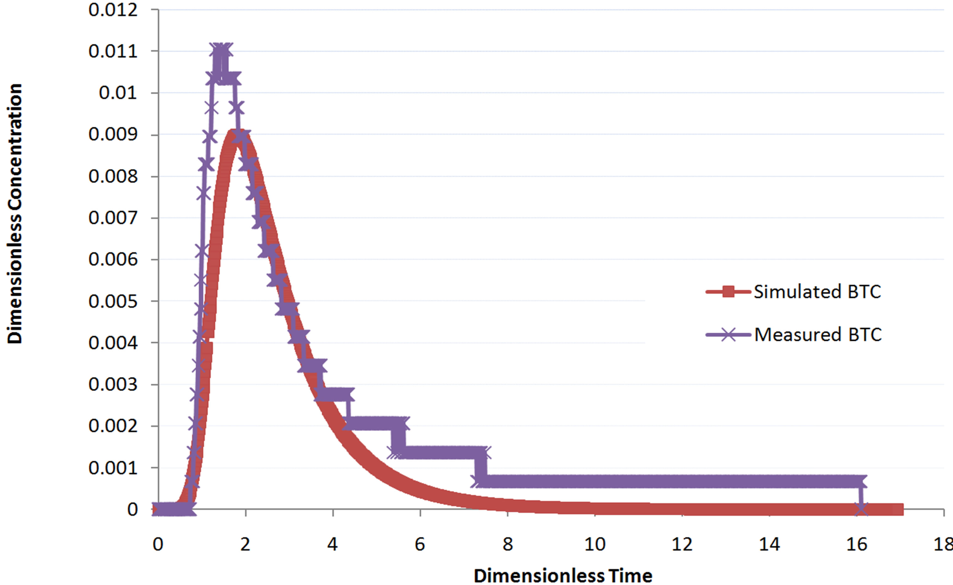
Figure 5. Observed and calculated breakthrough curve.
The two-dimensional Lattice Boltzmann model yielded a reasonable fit with the measured breakthrough curve and may be applied for larger scale in future research. The result presented should be considered carefully because the full picture about fractures geometry is not considered and a significant difference between measured and calculated BTC appeared for the tailing. More reliable result will be obtained after gaining more details about the geometry of the aquifer system. The major conclusion is that LBM as a rather new technique may be a good option to simulate the fluid flow and solute transport in fractured aquifers. Finally, coupling LBSim with PEST or UCODE will be a good option in the future to improve the result and acquire an automatic parameter estimation.
8. ACKNOWLEDGEMENTS
The authors wish to thank Fabio Sussumu Komori, Michael Sukop, and Timm Krüger for technical support in LBM. Also, we would like to thank Rudy Abo, Mohamed Omar, Weal Kanua, Raged Saber, and Marwa Emam for field test support. I am grateful for Dr. Mahmoud Bakr and Prof. Ali Subyani for encouraging and supporting. Also, we want to thank the anonymous reviewers for the valuable Comments and suggestions. This work has been supported by the Department of Hydrogeoloy at TU Freiberg.
REFERENCES
- Käss, W., Behrens, H., Himmelsbach, T. and Hötzl, H. (1998) Tracing technique in geohydrology. Balkema, Rotterdam, 581.
- Bodin, J., Delay, F. and De Marsily, G. (2003) Solute transport in a single fracture with negligible matrix permeability: 1. Fundamental mechanisms. Hydrogeology Journal, 11, 418-433. doi:10.1007/s10040-003-0268-2
- Leibundgut, C., Maloszewski, P. and Külls, C. (2011) Tracers in hydrology. John Wiley and Sons, Ltd., Hoboken.
- Schwartz, F.W. and Zhang, H. (2003) Fundamentals of ground water. John Wiley and Sons, Ltd., Hoboken.
- Singhal, B.B.S. and Gupta, R.P. (2010) Applied hydrogeology of fractured rocks. 2nd Edition, Springer, Berlin. doi:10.1007/978-90-481-8799-7
- Garabedian, S.P., LeBlanc, D.R., Gelhar, L.W. and Celia, M.A. (1991) Large-scale natural gradient tracer test in sand and gravel, Cape Cod, Massachusetts: 2. Analysis of spatial moments for a nonreactive tracer. Water Resources Research, 27, 911-924. doi:10.1029/91WR00242
- LeBlanc, D.R., Garabedian, S.P., Hess, K.M., Gelhar, L. W., Quadri, R.D., Stollenwerk, K.G. and Wood, W.W. (1991) Large-scale natural-gradient tracer test in sand and gravel. Cape Cod, Massachusetts: 1. Experimental design and observed tracer movement. Water Resources Research, 27, 895-910. doi:10.1029/91WR00241
- Adams, E.E. and Gelhar, L.W. (1992) Field study of dispersion in a heterogeneous aquifer: 2. Spatial moments analysis. Water Resources Research, 28, 3293-3307. doi:10.1029/92WR01757
- Rehfeldt, K.R., Boggs, J.M. and Gelhar, L.W. (1992) Field study of dispersion in a heterogeneous aquifer: 3. Geostatistical analysis of hydraulic conductivity. Water Resources Research, 28, 3309-3324. doi:10.1029/92WR01758
- Hess, K.M., Wolf, S.H. and Celia, M.A. (1992) Largescale natural gradient tracer test in sand and gravel, Cape Cod, Massachusetts: 3. Hydraulic conductivity variability and calculated macrodispersivities. Water Resources Research, 28, 2011-2027. doi:10.1029/92WR00668
- Sudicky, E.A. (1986) A natural gradient experiment on solute transport in a sand aquifer: Spatial variability of hydraulic conductivity and its role in the dispersion process. Water Resources Research, 22, 2069-2082. doi:10.1029/WR022i013p02069
- Abdelaziz, R. and Merkel, B.J. (2012) Analytical and numerical modeling of flow in a fractured gneiss aquifer. Journal of Water Resource and Protection, 4, 657-662. doi:10.4236/jwarp.2012.48076
- Slichter, C.S. (1905) Field measurements of the rate of movement of underground waters. United States Geological Survey Water-Supply and Irrigation Paper, 140, 711218.
- Bear, J., Tsang, C.F. and Marsily, G.D. (1993) Flow and contaminant transport in fractured rocks. Academic Press, San Diego.
- Gerke, H.H. and Van Genuchten, M.T. (1993) A dualporosity model for simulating the preferential movement of water and solutes in structured porous media. Water Resources Research, 29, 305-319. doi:10.1029/92WR02339
- Gerke, H.H. and Van Genuchten, M.T. (1993) Evaluation of a first-order water transfer term for variably saturated dual-porosity flow models. Water Resources Research, 29, 1225-1238. doi:10.1029/92WR02467
- Zhang, D. and Sun, A.Y. (2000) Stochastic analysis of transient saturated flow through heterogeneous fractured porous media: A double-permeability approach. Water Resources Research, 36, 865-874. doi:10.1029/2000WR900003
- Hu, B.X., Huang, H. and Zhang, D. (2002) Stochastic analysis of solute transport in heterogeneous, dual-permeability media. Water Resources Research, 38, 14-1- 14-16. doi:10.1029/2001WR000442
- Qian, Y.H., d’Humieres, D. and Lallemand, P. (2007) Lattice BGK models for Navier-Stokes equation. EPL (Europhysics Letters), 17, 479. doi:10.1209/0295-5075/17/6/001
- Chen, H., Chen, S. and Matthaeus, W.H. (1992) Recovery of the Navier-Stokes equations using a lattice-gas Boltzmann method. Physical Review A, 45, R5339-R5342. doi:10.1103/PhysRevA.45.R5339
- Chen, S., Martinez, D. and Mei, R. (1996) On boundary conditions in lattice Boltzmann methods. Physics of Fluids, 8, 2527. doi:10.1063/1.869035
- Flekkøy, E.G. (1993) Lattice Bhatnagar-Gross-Krook models for miscible fluids. Physical Review E, 47, 4247- 4257. doi:10.1103/PhysRevE.47.4247
- Gutfraind, R. and Hansen, A. (1995) Study of fracture permeability using lattice gas automata. Transport in Porous Media, 18, 131-149. doi:10.1007/BF01064675
- Yeo, W. (2001) Effect of fracture roughness on solute transport. Geosciences Journal, 5, 145-151. doi:10.1007/BF02910419
- He, X., Doolen, G.D. and Clark, T. (2002) Comparison of the lattice Boltzmann method and the artificial compressibility method for Navier-Stokes equations. Journal of Computational Physics, 179, 439-451. doi:10.1006/jcph.2002.7064
- Yoshino, M. and Inamuro, T. (2003) Lattice Boltzmann simulations for flow and heat/mass transfer problems in a three-dimensional porous structure. International Journal for Numerical Methods in Fluids, 43, 183-198. doi:10.1002/fld.607
- Zhang, X. and Ren, L. (2003) Lattice Boltzmann model for agrochemical transport in soils. Journal of Contaminant Hydrology, 67, 27-42. doi:10.1016/S0169-7722(03)00086-X
- Succi, S. (2001) The Lattice Boltzmann equation for fluid dynamics and beyond. Oxford University Press, New York.
- Sukop, M.C. and Thorne, D.T. (2006) Lattice Boltzmann modeling. Springer, Berlin.
- Field, M.S. (2002) The QTRACER2 program for tracerbreakthrough curve analysis for tracer tests in karstic aquifers and other hydrologic systems. National Center for Environmental Assessment—Washington Office, Office of Research and Development, US Environmental Protection Agency, Washington DC.
- Tam, V.T., Vu, T.M.N. and Batelaan, O. (2001) Hydrogeological characteristics of a cast mountainous catchment in the northwest of Vietnam. Acta Geologica Sinica— English Edition, 75, 260-268. doi:10.1111/j.1755-6724.2001.tb00529.x
- Birk, S., Geyer, T., Liedl, R. and Sauter, M. (2005) Process- based interpretation of tracer tests in carbonate aquifers. Groundwater, 43, 381-388. doi:10.1111/j.1745-6584.2005.0033.x
- Massei, N., Wang, H.Q., Field, M.S., Dupont, J.P., Bakalowicz, M. and Rodet, J. (2006). Interpreting tracer breakthrough tailing in a conduit-dominated karstic aquifer. Hydrogeology Journal, 14, 849-858. doi:10.1007/s10040-005-0010-3
- Gabrovšek, F., Kogovšek, J., Kovačič, G., Petrič, M., Ravbar, N. and Turk, J. (2010) Recent results of tracer tests in the catchment of the Unica river (sw slovenia). Acta Carsologica, 1, 39.
- Bear, J. (1979) Hydraulics of groundwater, McGraw-Hill series in water resources and environmental engineering. McGraw-Hill, New York.
- He, X. and Luo, L.S. (1997) A priori derivation of the lattice Boltzmann equation. Physical Review E, 55, 6333- 6336. doi:10.1103/PhysRevE.55.R6333
- Sukop, M.C., Anwar, S., Lee, J.S., Cunningham, K.J. and Langevin, C.D. (2008) Modeling ground-water flow and solute transport in karst with lattice Boltzmann methods. In Proceedings of the US Geological Survey Karst Interest Group Workshop, Bowling Green, 27-29 May 2008, 77-86.
- Lee, J.Y. and Lee, K.K. (2000) Use of hydrologic time series data for identification of recharge mechanism in a fractured bedrock aquifer system. Journal of Hydrology, 229, 190-201. doi:10.1016/S0022-1694(00)00158-X
- Shook, G.M., Ansley, S.L. and Wylie, A. (2004) Tracers and tracer testing: Design, implementation, and interpretation methods. Idaho National Engineering and Environmental Laboratory, Idaho Falls. www.inl.gov/technicalpublications/Documents/2603379.pdf doi:10.2172/910642
- Field, M.S. (1999) The QTRACER program for tracerbreakthrough curve analysis for karst and fractured-rock aquifers. National Center for Environmental Assessment— Washington Office, Office of Research and Development, US Environmental Protection Agency, Washington DC.
- Field, M.S. and Pinsky, P.F. (2000) A two-region nonequilibrium model for solute transport in solution conduits in karstic aquifers. Journal of Contaminant Hydrology, 44, 329-351. doi:10.1016/S0169-7722(00)00099-1
- Anwar, S. (2008) Lattice Boltzmann modeling of fluid flow and solute transport in karst aquifers. FIU Electronic Theses and Dissertations, Florida International University, University Park.
- Anwar, S. and Sukop, M.C. (2009) Lattice Boltzmann models for flow and transport in saturated karst. Groundwater, 47, 401-413. doi:10.1111/j.1745-6584.2008.00514.x
- Komori, F.S., Mielli, M.Z. and Carreño, M.N. (2011) Simulator for microfluidics based on the lattice Boltzmann method. ECS Transactions, 39, 461-468. doi:10.1149/1.3615227
- Komori, F.S. (2012) Development of a simulator computational fluid dynamics using the lattice Boltzmann method. M.Sc. Theses, University of São Paulo, São Paulo.
- Fetter, C.W. (2008) Contaminant hydrogeology. 2nd Edition, Waveland Press, Inc., Long Grove.