Health
Vol. 4 No. 3 (2012) , Article ID: 18338 , 4 pages DOI:10.4236/health.2012.43024
Dynamics of firm size in healthcare industry
![]()
Swiss Federal Institute of Technology, Lausanne, Switzerland; Fariba.Hashemi@epfl.ch
Received 2 September 2011; revised 12 October 2011; accepted 3 November 2011
Keywords: Firm Size Heterogeneity; Healthcare; Pharmaceuticals; Biotechnology; Industry Dynamics; Stochastic Analysis
ABSTRACT
Healthcare is one of the world’s fastest growing industries consisting of broad services offered by various hospitals, physicians, nursing homes, diagnostic laboratories, pharma-cies and supported by drugs, pharmaceuticals, chemicals, medical equipment, manufactu-rers and suppliers. The industry is highly fragmented, comprising of various ancillary sectors namely medical equipment and supplies, pharmaceutical, healthcare services, biotechnology, and alternative medicines. The present study focuses on the pharmaceu-tical and biotechnology segments of the healthcare industry, and presents a stochastic analysis of the evolution over time of firm size. A dynamic model is proposed that attempts to predict the evolutionary process of firm size distribution based on industry and product characteristics. A validation exercise, applying the model to pharmaceutical and the biotechnology industries finds that the predictions from the model are very close to the actual trajectories of firm size distributions within these industries at the global level. The results show interestingly, that the drivers of firm size dynamics are industry level characteristics that can be estimated from historical data with some accuracy. Specifically, it is found that firm size distributions are approaching a long-run equilibrium at a faster rate in the case of the pharmaceutical industry and that the dispersion of the distributions are shrinking over time above all for the biotechnology industry.
1. INTRODUCTION
The distribution of firm size has enjoyed a privileged position in the Industrial Organization literature. Since the earliest contributions, attention has focused on the explanation of the shape of firm size distribution at a given point in time by reference to steady state arguments. The dynamics in question have been relatively ignored however. The main objective of this paper is to help fill this gap by introducing a stochastic model that allows to incorporate dynamics which are typically neglected when looking at distribution of firm sizes. We consider a representation for the dynamics in the evolving distributions where the growth distribution of firm sizes can be generated by a single stochastic process in which firm size follows a Brownian motion. A crossindustry empirical analysis, comparing dynamics of firm size in Pharmaceutical and Biotechnology industries fills a second gap in the literature, as only few diffusion studies have employed real statistical data when analyzing firm size dynamics. The applicability of the proposed method suggests that diffusion may be a preferable technique for the analysis of spatial dynamics in firm size. It is a more transparent way to quantify dynamics, as it avoids the complications associated with dynamic inference and statistical regression fallacy inherent in standard cross-section tests [1-3].
The paper is organized as follows: Section 2 provides a theoretical framework. Section 3 discusses the relation of this study to the previous literature. Section 4 presents the model and Section 5, the empirical application. Section 6 concludes with suggested directions for future research.
2. THEORETICAL FRAMEWORK
The study is motivated by the observation that the distribution of size of firms varies over time, both within and across industries. A question of both theoretical and empirical importance is drivers of industry dynamics. To examine this question, we propose a classical stochastic model for the evolution of cross-sectional distribution of firm size around its trend. The model is mechanical and descriptive in nature. It describes the diffusion of shocks across space, via an adjustment process with noise. The dynamics of the model rely on two counteracting flows: 1) a mean reversion process and 2) a diffusion process. Noise is generated by a search and learning process, based on imitation, trial and error, and learning-by-doing behavior à la Arrow [4], Nelson and Winter [5], and Levine [6]. It is hypothesized that these flows follow simple evolutionary laws that can be described with five parameters.
3. RELATION TO PREVIOUS LITERATURE
Although the process proposed in this paper is compatible with σ and β convergence type specifications in the literature on firm size [7-19], it adopts a different approach. Amongst the studies on distribution of firm sizes, only a select few have attempted to examine its evolution either at the industry or at the economy-wide level. Cabral and Mata [20] pioneered an evolutionary approach to explain the firm size distribution and showed that the distribution of the logarithms of firm size of young cohorts are skewed, but the distribution gradually moves towards a lognormal distribution in older cohorts. The authors show that most of the observed changes in the firm size distribution results from the evolution of the distribution of survivors of a given cohort, and are not due to firm selection processes. Theories such as Jovanovic [9], Hopenhayn [11], and Ericson and Pakes [21] are often cited to motivate firm turnover in young firms [19]. The emphasis of Cabral and Mata [20] is on the evolution of the distribution of survivors of a given cohort and not on noisy selection (i.e. not on entry and exit in young cohorts). The innovation in the present paper is to take the ideas of learning from Jovanovic [9], Hopenhayn [11] and Ericson and Pakes [21] but apply them to the evolution of size in surviving incumbent firms. In other words, is the learning process that is driving the effect age overtime in the firm size distribution. Hutchinson, Konings and Walsh [19] expand the idea of Cabral and Mata [20] to explore whether time to build product portfolios can be proxy for age of companies and how it may impact the firm size distribution. The present analysis is consistent with Hutchinson, Konings and Walsh, but adds that trial and error is needed to create these segments of the market in the first place. Outcome of such learning processes moves the firm size distribution along and gives the dynamic structure certain properties that are industry specific. Hence the paper promotes modeling of the drivers of industry dynamics without having to derive a steady state solution. Cabral and Mata [20] and Hutchinson, Konings, Walsh [19] already do this. This paper adds a little more structure to this kind of approach.
4. THE MODEL
Consider an industry consisting of a constant number of firms with different sizes. Firm size is distributed as log-normal. Average costs of producing an amount x of output are a non-increasing function of firm size for a given quality of output. Each firm may have significant fixed costs, and marginal costs may essentially be constant. Furthermore, consumers prefer small firms for perceived higher quality of service. Under these conditions, there would exist a limit equilibrium distribution of firm sizes with a certain unknown mean and variance, determined by the tension between economies of scale in production and consumer preference for smaller firms. The equilibrium trades off productive efficiency against consumer preferences, and the evolution of the distribution reflects convergence towards this equilibrium1.
The history of a firm is governed by an ordinary differential equation  where
where  is the drift. Letting
  be the solution such that
  , we get
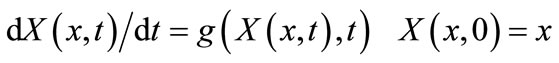 (1)
(1)
Assume that x > 0 and that the solution  remains positive (see Appendix A).
From the point of view of diffusion processes, consider a stochastic differential equation of the Ito type
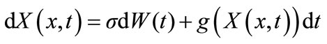 (2)
(2)
where σ is a small constant, and W is a standard Wiener process. Under mild conditions on g, Eq.2 is known to have a unique solution. Moreover, for each t > 0 and each x,  does have a probability density
  and
and  satisfies Kolmogorov’s forward equation.
Consider the form where u > 0. In this case, each point moves toward the position u but never reaches it. More precisely, for the drift spread, it is assumed that there exists some equilibrium distribution of firm sizes with a certain mean and variance, towards which the ensemble of firms gravitate. For the drift spread, bounded rationality, search and learning, trial and error and imitation generate noise in the system (Levine [6], Fudenberg and Levine [23]). Random effects tend to cause a spread of firms from regions of high density toward lower density sizes. The speed of spreading parameter, related to the adjustment process, is interpreted as depending on learning speed. This learning process generates randomness in the system.
Hence, assuming that firm size behaves like a stochastic process and that it is continuous and Markovian, we consider the most natural candidate; a classical linear stochastic differential equation driven by a standard Wiener process:
 (3)
(3)
where  is firm size. λ denotes the adjustment rate, assumed constant for simplicity. u denotes the mean of the stationary equilibrium distribution, σ is a small constant, and W(t) is a standard Wiener process.
Analysis of the Model
The process derived from the diffusion model evolves according to an Ornstein-Uhlenbeck. This type of model has been widely used in Biomathematics [26-30]. The Ornstein-Uhlenbeck is the most general normal stationary Markovian process with zero expectations. For t > T, the transition density from (T,s) to (t,y) is normal with expectation  and variance
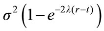 . As
. As , the expectation tends to 0 and the variance to
 . The analytic solution derived for our diffusion equation is a normal distribution for all t. There is the
  factor; with a change of variables, it can be shown that the solution is normal with a constant multiplied by it2.
5. EMPIRICAL APPLICATION
5.1. Data and Descriptive Statistics
The empirical analysis presents a cross-industry and cross-sectional analysis of the Biotechnology and Pharmaceuticals segments of the Healthcare industry. The empirical portion is conducted in three steps: In the first step, a cross-industry analysis is presented, where the proposed model is applied to the evolution of size distribution of two different segments of the Healthcare industry between the years 1989-2007: 1) Global Pharmaceuticals and 2) Global Biotechnology. In the second step, the model is applied to the evolution of firm size distribution for the US sub-segment of the two industries. The third step involves a cross-sectional analysis, focusing on the Pharmaceutical and Biotechnology industries in isolation, and comparing the Global and US portions of each.
Our first data describes the Global Pharmaceutical industry between the years 1989-2007. Pharmaceuticals are a relatively large and mature industry, and of growing significance. Its market size globally is around $700 billion, with a growth rate of 5 - 8 percent per year. The cost of bringing a new drug to market (including the cost of clinical trials and failures) is estimated at around $800 million in 2000 dollars. The global market is geographically concentrated, with sales in the US accounting for about 48% of the total, followed by Europe’s 29% and Japan’s 11%. Since the mid-eighties, the industry has gone through a wave of mergers and acquisitions which has made the industry more and more concentrated. This phenomenon has run parallel to the emergence of Biotechnology and Generics. Figure 1 provides a description of the evolution of the distribution of firm sizes in this data, where number of employees is used as proxy for firm size. Observations were available annually, and the sample includes 502 companies engaged in the research, development or production of Pharmaceuticals3.

Figure 1. Evolution in distribution of firm size for pharmaceuticals.
The vertical axis measures firm size in logarithms, and the horizontal axis measures time in years. The solid line represents the mean size of the industry and the dotted lines one standard deviation around the mean.
Our second data set describes the Global Biotechnology industry between the years 1989-2007. The sample consists of a total of 197 Biotechnology firms primarily engaged in research, development, manufacturing and/or marketing of products based on genetic analysis and genetic engineering. Observations were available annually. Figure 2 provides a description of the evolution of the distribution of firm sizes in this data, where our measure of firm size is once again, the total number of employees. The vertical axis measures firm size in logarithms, and the horizontal axis measures time in years. The solid line represents the mean size of the industry and the dotted lines, one standard deviation around the mean.
The model has five parameters: , and
, and 
 denotes the initial mean of the distribution, and u denotes the mean of the steady state distribution.
  is the initial variance,
  represents the strength of the diffusion effect, and
  represents the strength of the mean reversion effect. The model has been applied to the distribution of firm size for the two populations as a function of time. Table 1 reports estimates for the five model parameters, along with the standard errors and t-values.
Figures 3 and 4 graphically illustrate the mean of the firm size distribution in the Pharmaceutical and Biotechnology data respectively (dotted line), superimposed on the mean of the size distribution as predicted by the model (bold solid line, +/– one standard deviation). The vertical axis on this panel measures the mean of the size distribution (in logarithms) and the horizontal axis measures time in years.
Figures 5 and 6 graphically illustrate the standard deviation of the size distribution in the Pharmaceutical and Biotechnology industries respectively (dots), superimposed on the standard deviation of the respective distributions as predicted by the model (solid curves).
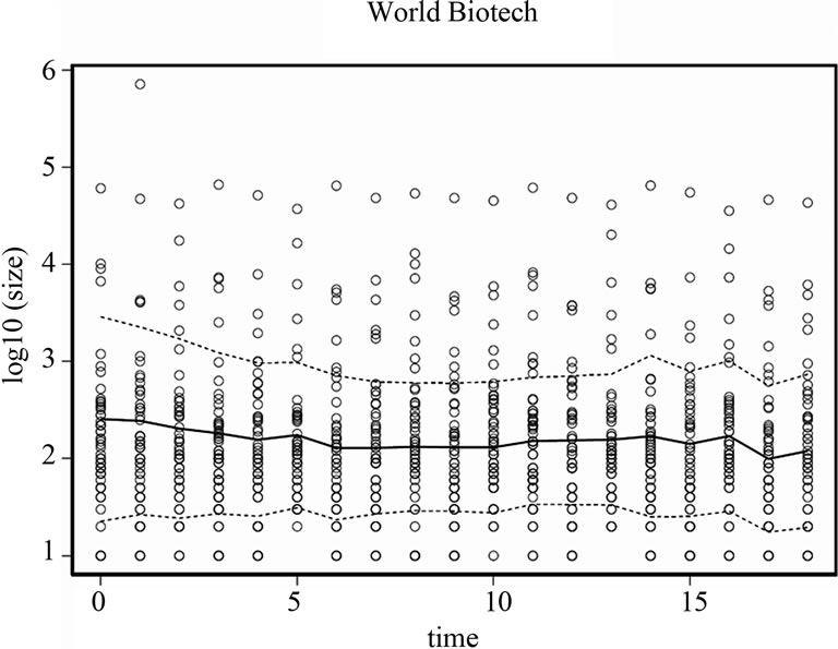
Figure 2. Evolution in distribution of firm size for biotechnology.
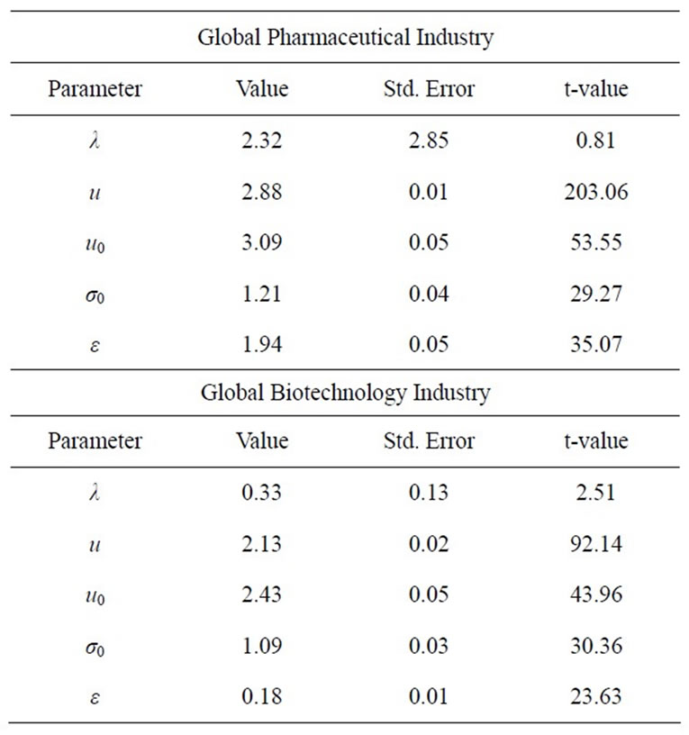
Table 1. Parameter estimates for global pharmaceutical and biotechnology industries.
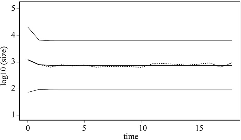
Figure 3. Mean of the distribution for pharmaceuticals.

Figure 4. Mean of the distribution for biotechnology.

Figure 5. Standard deviation of the distribution for pharmaceuticals.
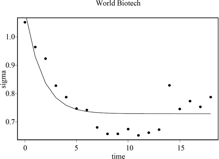
Figure 6. Standard deviation of the distribution for biotechnology.
To ascertain whether the parameter estimates conform to the real data presented in the descriptive analysis, Figures 7 and 8 illustrate the actual versus predicted
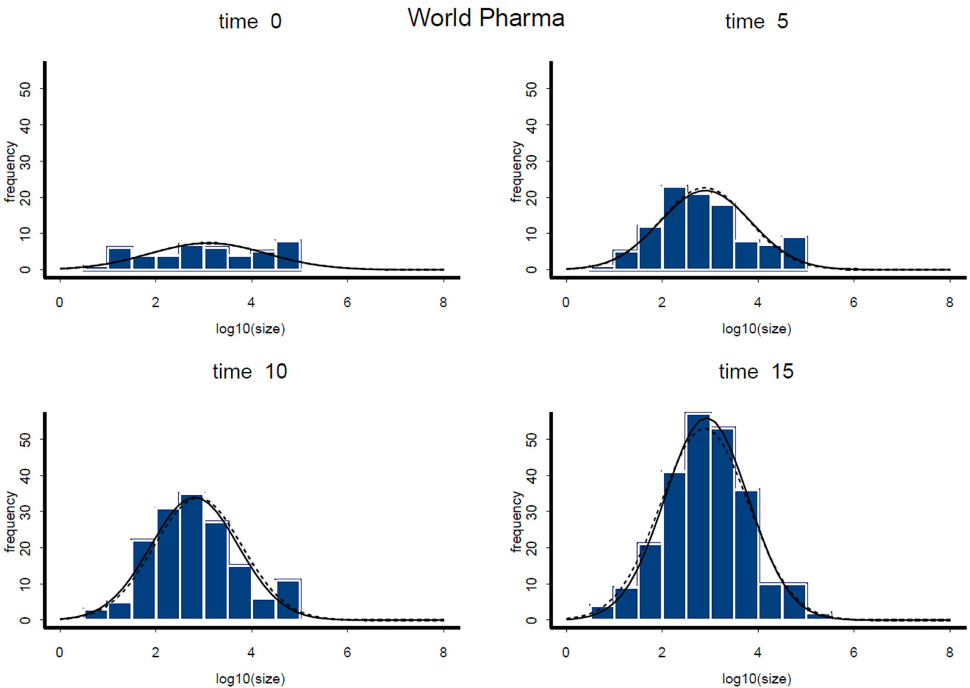
Figure 7. Predicted vs. actual distribution for pharmaceuticals.
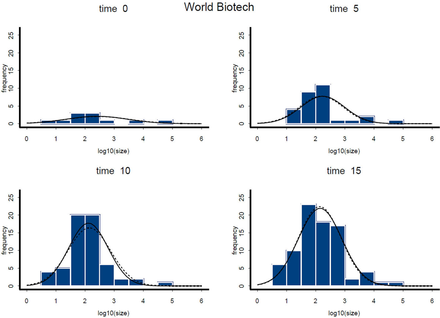
Figure 8. Predicted vs. actual distribution for biotechnology.
time plot that can be generated from the real and estimated data. These figures graphically illustrate the evolution of the firm size distribution (log-normals) over time for the Pharmaceutical and Biotechnology industries respectively, superimposed on histograms which describe the time evolution of the distribution of firm sizes in the data (for selected years). The solid curves in these figures illustrate the distribution of firm size as predicted by the model, and the dotted curves illustrate the distribution of firm size in the data. The vertical axes in these figures denote frequency, and the horizontal axes measure firm size in logarithms. These figures illustrate that the nice pattern which we see in the fitted log normals are being pulled out of a set of histograms whose shape are irregular.
The following observations can be made concerning our results:
1) The mean and variance of both distributions are clearly evolving, corresponding to our theoretical predictions.
2) The value for the strength of the mean reversion process , is small and positive and varies for the two industries, corresponding to our theoretical predictions. Mean reversion is stronger in the Pharmaceutical industry than in Biotechnology.
3) The value for the strength of the diffusion effect is likewise small and positive and varies from industry to industry, corresponding to our theoretical predictions. The diffusive limit is , which is larger for Pharmaceutical than for Biotechnology, suggesting a slightly more homogeneous firm size within the later. The results predict that if we start with a normal distribution and let the model drive the distribution, the distribution variance will tend toward a constant
 , and concentrated around a mean u which is larger for Pharmaceutical than for Biotechnology.
5.2. Empirical Application to the US Segments of the Two Industries
In the following section, we present a cross-industry analysis of the US data, comparing US Pharmaceutical and US Biotechnology, followed by an analysis of each industry in isolation, comparing the US and its Global counterparts. Table 2 reports estimates for the five model parameters 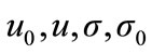 and
and , along with the standard errors and t-values for each industry respectively.
Figures 9 and 10 graphically illustrate the evolution of the firm size distribution (log-normals) over time for the US Pharmaceutical and US Biotechnology industries respectively, superimposed on histograms which describe the time evolution of the distribution of firm sizes in the data (for selected years). The solid curves in these figures illustrate the distribution of firm size as predicted by the model, and the dotted curves illustrate the distri-

Table 2. Parameter estimates for US pharmaceutical and US biotechnology industries.
bution of firm size in the data. The vertical axes in these figures denote frequency, and the horizontal axes measure firm size in logarithms. These figures illustrate that the nice pattern which we see in the fitted log normals are being pulled out of a set of histograms whose shape are irregular.
Table 3 summarizes the findings for the four subpopulations. The following observations can be made concerning our results:
1) The mean and variance of both distributions are clearly evolving, corresponding to our theoretical predictions.
2) The value for the strength of the mean reversion process , is small and positive and varies from industry to industry, corresponding to our theoretical predictions.
3) The value for the strength of the diffusion effect is likewise small and positive and varies from industry to industry. The diffusive limit is larger in Pharmaceutical industry than in Biotechnology, suggesting a more homogeneous firm size in the later. This result conforms to our earlier finding regarding the Global cohort of the two industries.
We observe a marked difference between the two industries in the dynamic adjustment to stationary equilibrium and in the dispersion of the size distributions. This comes as no surprise, and indicates differences between the two industries, with respect to their size, product characteristics, stage of growth, and competition. The field of modern biotechnology is thought to have largely begun in 1980, when the United States Supreme Court ruled that a genetically-modified microorganism could be
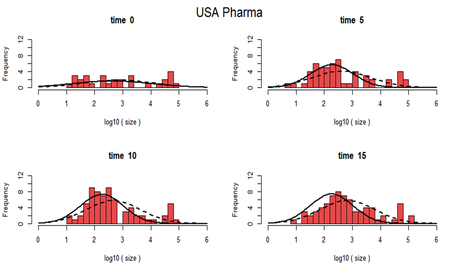
Figure 9. Actual versus Predicted Distributions in Pharmaceuticals.

Figure 10. Actual versus Predicted Distributions in Biotechnology.
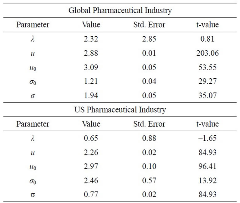

Table 3. Parameter estimates for US and global pharmaceutical and biotechnology industries.
patented. Pharmaceuticals however, represent a relatively large and mature segment of the Global Healthcare industry. Most of today’s major Pharmaceutical companies were founded in the late 19th and early 20th centuries. The industry remained relatively small scale until the 1970s when it began to expand at a greater rate. It entered the 1980s pressured by economics and a host of new regulations, and transformed by new DNA chemistries and new technologies. A new business atmosphere became institutionalized during the last two decades where the Pharmaceutical industry underwent extensive restructuring in the form of mergers and acquisitions. The dynamic process proposed in this paper requires a wide enough variety of strategies and actions that have already been experimented with, which is more plausible for larger, more mature, and relatively heterogeneous industries, than for smaller, relatively younger, and relatively homogeneous industries, which to some extent display the features of Sutton’s [33] “strategic dependence” hypothesis of homogeneous submarkets. Sutton puts forward the idea that firm heterogeneity in the collection of sub-markets (product lines or geographical areas) during industry evolution is a core determinant of the firm size distributions. As firms learn passively, they must represent a sufficient variety of behaviors such that as Alchian [34] famously noted”... what really counts is the various actions actually tried, for it is from these that success is selected, not from some set of perfect actions” [34, p. 220]. One might thus expect the rates of learning and dynamic adjustment to stationary equilibrium to be rather slow in a relatively small, young and homogeneous industry where competition is relatively week and trial and error and imitation are limited. Our empirical results suggest that this might indeed be the case.
6. CONCLUSIONS
By considerations of analytic tractability, the model developed in this paper is simplified. The dynamics represent a trade-off between a preference for small size on the part of the consumers and a technological advantage of being large, but the dynamics could represent many other forces as well. Small firms may be able to adapt to changes in the environment more easily, and large firms may have higher visibility and may thus benefit from reputation effects. Moreover, both the Pharmaceutical and the Biotechnology industries are governed by a rich set of environmental, political, and institutional characteristics. For instance, the Pharmaceutical industry faces extremely different regulatory frameworks from country to country, and these regulations suffer drastic changes very often. Some of the dispersion in firm size one sees in the Global Pharmaceutical market could be driven by the location of the Pharmaceutical firms or by the particular markets where they are currently present. Moreover, in this paper, number of employees has been selected as proxy for firm size realizing that for technological and research industries such as Pharmaceuticals and Biotechnology, there are additional measures one could use. On this, I have built on earlier literature on firm size where size had been proxied by sales, income, number of employees, or total assets (Simon and Bonini [35], Ijiri and Simon [8], Sutton [33], Axtell [14] and Hutchinson et al. [19]). An interesting property of firm size distributions noted in previous studies of large firms is that the qualitative character of such distributions is independent of how size is defined (Axtell [14]).
Furthermore, the model presented in this paper includes no exogenous control variables that shift the conditional mean (e.g. business cycle effects). An extension which would significantly enrich the present analysis would be to include such exogenous control variables. We also observe that the rate of approach to final equilibrium, as well as the relaxation time in our model only depend on λ characterizing the drift term, but does not depend on the diffusion strength. This feature is entirely inherent to the linearity of the dynamics considered in this paper and turns out to be a limitation in the modeling capability offered by Ornstein-Uhlenbeck. For nonlinear drifts, this feature does not occur anymore and the rate of approach to final equilibrium may strongly depend on the diffusion parameter, and as such, the noise strength strongly affects the transient behavior of the probability density.
In general, an exercise such as the one presented in this paper is informative from the point of view of understanding industry dynamics and shaping policy. The methodology proposed in this paper can be extended to formally map industry characteristics on the dynamics of firm structure, to predict the evolutionary process of firm size distribution based on industry and product characteristics. One area of investigation which would prove informative is patents. This is important because in circumstances where innovations build on each other— which is the case for the discovery and development of both biologics and drugs—patents can be especially costly, as they may reduce rather than encourage the incentive to innovate. As early as in the early seventies, Hirshleifer [36] theoretically illustrated that economically valuable information can be traded in the absence of patents and under condition of competition. More recently, Boldrin and Levine [37,38] have shown that there is no theoretical need to postulate either increasing returns or monopoly power to understand the dynamics of innovation in Pharmaceuticals, and that the traditional competitive model provides a more solid foundation for the examination of R&D processes in this industry. A good understanding of which kind of characteristics lead to which kinds of dynamics helps us understand how incentives should be provided for the socially optimal amount of creative activity to take place. Given the current R&D slowdown in both Pharmaceutical and Biotechnology industries, this seems to be a most valuable direction for future research, with critical implications for the future of Global Healthcare.
7. ACKNOWLEDGEMENTS
The author acknowledges and thanks Omega statistical consulting for assistance in the statistical analysis of this paper. This paper builds on previous work of the author [39-40].
![]()
![]()
REFERENCES
- Friedman, M. (1992) Do old fallacies ever die? Journal of Economic Literature, 30, 2129-2132.
- Quah, D. (2003) Empirics for economic growth and convergence. The Economics of Structural Change, Elgar Reference Collection, 3, 174-196.
- Kevin, L., Pesaran, H. and Smith, R. (1998) Growth empirics: A panel data approach—A comment. Quarterly Journal of Economics, 113, 319-323. doi:10.1162/003355398555504
- Arrow, K.J. (1962) The economic implications of learning-by-doing. Review of Economic Studies, 29, 155.
- Nelson, R.R. and Winter, S.G. (1982) An evolutionary theory of economic change. Harvard University Press, Cambridge.
- Levine, D. (2011) Neuroeconomics? International Review of Economics, 58, 287-305. doi:10.1007/s12232-011-0128-7
- Gibrat, R. (1931) Les inegalite economiques. Sirey, Paris.
- Ijiri, Y. and Simon, H.A. (1977) Interpretations of departures from the pareto curve firm-size distributions. Journal of Political Economy, 82, 315-331.
- Jovanovic, B. (1982) Selection and the evolution of industry. Econometrica, 50, 649-670. doi:10.2307/1912606
- Simon, H.A. (1997) Models of bounded rationality: Empirically grounded economic reason. 3, The MIT Press, Cambridge.
- Hopenhayn, H. (1992) Entry, exit, and firm dynamics in long run equilibrium. Econometrica, 60, 1127-1150. doi:10.2307/2951541
- Stanley, M.H.R., et al. (1996) Scaling behaviour in the growth of companies. Nature, 319, 804-806.
- Sutton, J. (1997) Gibrats legacy. Journal of Economic Literature, 35, 4059.
- Axtell, R. (2001) Zipf distribution of US firm sizes. Science, 293, 1818-1820. doi:10.1126/science.1062081
- Lotti, F. and Santarelli, E. (2004) Industry dynamics and the disrtribution of firm sizes. Southern Economic Journal, 70, 443-466. doi:10.2307/4135325
- Klepper, S. and Thompson, P. (2006) Submarkets and the evolution of market structure. Rand Journal of Economics, 37, 861-886. doi:10.1111/j.1756-2171.2006.tb00061.x
- Luttmer, E. (2007) Selection, Growth, and the size distribution of firms. Quarterly Journal of Economics, 122, 1103-1144. doi:10.1162/qjec.122.3.1103
- Angelini, P. and Generale, A. (2008) On the evolution of firm size distributions. American Economic Review, 98, 426-438. doi:10.1257/aer.98.1.426
- Hutchinson, J., Konings, J. and Walsh, P.P. (2010) The firm size distribution and inter-industry diversification. Review of Industrial Organization, 37, 65-82. doi:10.1007/s11151-010-9260-x
- Cabral, L. and Mata, J. (2003) On the evolution of the firm size distribution: Facts and theory. American Economic Review,
- Pakes, A. and Ericson, R. (1998) Empirical implications of alternative models of firm dynamics. Journal of Economic Theory, 79, 1-45.
- Chamberlin, E. (1933) Theory of monopolistic competition. Harvard University Press, Cambridge.
- Robinson, J. (1933) The economics of imperfect competition. Macmillan, London.
- Spence, M. (1976) Product selection, fixed costs, and monopolistic competition. Review of Economic Studies.
- Dixit, A. and Stiglitz, J. (1977) Monopolistic competition and optimal product diversity. American Economic Review, 67, 297-308.
- Hongler, M.-O., Filliger, R. and Blanchard, P. (2006) Soluble models for dynamics driven by a super-diffusive noise. Physica, 370, 301-315.
- Hongler, M.-O., Soner, H. and Streit, L. (2004) Stochastic control for a class of random evolution models. Applied Mathematics and Optimization, 49, 113-121.
- Besson, O. and de Montmollin, G. (2004) Space-time integrated least squares: A time-marching approach. International Journal for Numerical Methods in Fluids, 44, 525-543. doi:10.1002/fld.655
- Harris, T. (1963) The theory of branching processes. Springer-Verlag, Berlin.
- Harris, T. (1974) Contact interactions on a lattice. Annals of Probability, 2, 969-988. doi:10.1214/aop/1176996493
- Hashemi, F. (2003) A dynamic model of size distribution of firms applied to US biotechnology and trucking industries. Small Business Economics, 21, 27-36. doi:10.1023/A:1024433203253
- Hashemi, F. (2000) An evolutionary model of the size distribution of firms. Journal of Evolutionary Economics, 10, 507-521. doi:10.1007/s001910000048
- Sutton, J. (1998) Technology and market structure: Theory and history. MIT Press, Cambridge.
- Alchian, A.A. (1950) Uncertainty, evolution, and economic theory. Journal of Political Economy, 58, 211-221.
- Simon, H.A. and Bonini, C.P. (1958) The size distribution of business firms. American Economic Review, 48, 607- 617
- Hirshleifer, J. (1971) The private and social value of information and the reward to inventive activity. American Economic Review, 61, 561-574.
- Boldrin, M. and Levine, D. (2009) A model of discovery. American Economic Review, 99, 337-342. doi:10.1257/aer.99.2.337
- Boldrin, M. and Levine, D. () What’s intellectual property good for? Revue Economique, Forthcoming.
- Hashemi, F. (2012) Industry Dynamics in Pharmaceuticals,Pharmacology and Pharmacy, 3, 1-6 doi: 10.4236/pp.2012.31001
- Hashemi, F. (2012) Industry Dynamics in Biotechnology,Advances in Bioscience and Biotechnology, 3, 35-39. doi: 10.4236/abb.2012.31006
Appendix A
Remark 1
This is a degenerate diffusion with no Brownian noise. Thus the position at time t of a firm size starting at x does not have a probability density in the ordinary sense but is deterministic. It is important that a differential equation such as (1) defines a flow on the whole interval . In other words, a set in
  for example an interval (a,b), is transformed into the interval (X(a,t)) (X(b,t)) at time t. Assuming g(x,t) is a “reasonable” function, the paths from two distinct points, namely
  and
and  will never meet, so an interval remains an interval under this flow. The flow transforms any initial measure on the interval
  into a different measure. Suppose the initial measure is given by a density function
 , where we can normalize by taking
  Then the transformed measure attaches to the interval (a,b) the measure

 , where
  and
and  (which depend on t ) are the inverse images of a and b:
 ,
, . Assuming that g is not very peculiar and the transformed measure also has a density, call the transformed density
 . One can interpret
  as the mass density at time t; alternatively, if we think of
  as the initial probability density for a single firm, then
  is the probability density at time t. For the mass density interpretation, we may think of

 as the fraction of all firms that are in the interval
  at time t. Our picture of the world thus follows the lines of the derivation used for Kolmogorov’s forward differential equation. Taking the probability interpretation, with the initial density
 , let
, let  be the randomized X-process, using
  for the vanishing of some finite subinterval of
Remark 2
In Eq.2, x is fixed, indicating the starting point.  is a Dirac function, with all the mass concentrated at x, and so is not a density in the ordinary sense. For t > 0, one has Prob
We may again suppose x is initially random.
NOTES
1This tension goes back to Chamberlin’s and Robinson’s ideas of “monopolistic competition”, and was formalized by Spence and DixitStiglitz [see 22-25].
2Ref [31,32] develop and provide a full analysis of this model, albeit in a different context.
3The data set includes 502 companies comprising the universe of all firms in the Pharmaceutical industry, and 197 companies comprising the universe of all firms in the Biotechnology industry.