Engineering
Vol.5 No.10A(2013), Article ID:38449,11 pages DOI:10.4236/eng.2013.510A007
Wind Power Uncertainty and Power System Performance
1Departmentof Biological and Environmental Engineering, Cornell University, Ithaca, USA
2Picker Engineering Program and Department of Computer Science, Smith College, Northampton, USA
Email: jcardell@smith.edu
Copyright © 2013 C. Lindsay Anderson, Judith B. Cardell. This is an open access article distributed under the Creative Commons Attribution License, which permits unrestricted use, distribution, and reproduction in any medium, provided the original work is properly cited.
Received July 31, 2013; revised August 31, 2013; accepted September 7, 2013
Keywords: Wind Power; Power System Operations; Variable Energy Resources; Demand Response
ABSTRACT
The penetration of wind power into global electric power systems is steadily increasing, with the possibility of 30% to 80% of electrical energy coming from wind within the coming decades. At penetrations below 10% of electricity from wind, the impact of this variable resource on power system operations is manageable with historical operating strategies. As this penetration increases, new methods for operating the power system and electricity markets need to be developed. As part of this process, the expected impact of increased wind penetration needs to be better understood and quantified. This paper presents a comprehensive modeling framework, combining optimal power flow with Monte Carlo simulations used to quantify the impact of high levels of wind power generation in the power system. The impact on power system performance is analyzed in terms of generator dispatch patterns, electricity price and its standard deviation, CO2 emissions and amount of wind power spilled. Simulations with 10%, 20% and 30% wind penetration are analyzed for the IEEE 39 bus test system, with input data representing the New England region. Results show that wind power predominantly displaces natural gas fired generation across all scenarios. The inclusion of increasing amounts of wind can result in price spike events, as the system is required to dispatch down expensive demand in order to maintain the energy balance. These events are shown to be mitigated by the inclusion of demand response resources. Benefits include significant reductions in CO2 emissions, up to 75% reductions at 30% wind penetration, as compared to emissions with no wind integration.
1. Introduction
The installed capacity of wind power plants throughout the world is gradually increasing, in response to pressure for developing lower emitting generating technologies as well as an interest in capturing the energy available in the vast wind resource. In many regions, the penetration level remains low enough that significant impacts from the intermittent nature of the wind resource are not yet realized. However, in regions with higher penetration of wind power capacity, the intermittent behavior of wind power requires power system planners and operators to develop new methods and tools to reliably integrate wind into their systems [1-5].
There exist empirical studies that quantify the impacts from existing wind power plant installations [6,7]. These studies analyze actual wind events, such as sudden changes in wind power generation, their impact on system behavior, and possible methods for minimizing these impacts.
This paper presents an analysis of the expected system behavior over a more complete range of possible wind events and other system contingencies through Monte Carlo simulation. The analysis and results are intended to be useful to system planners and operators in better understanding the probability of worst-case scenarios, and their impacts on system and market operations. The results also quantify the impact of wind variability on system performance parameters such as generator dispatch patterns, CO2 emissions, and the electricity price (locational marginal price, or LMP) by estimation of the empirical distribution for these impacts.
A major effort in this project is the development of the modeling framework, which is presented in Section 2. Section 3 discusses modeling three sources of uncertainty in power system operations: wind forecasts, load forecast and generator availability. Section 4 presents the power system test model used in the simulations, including the simplified transmission system and generator technology mix. Section 5 briefly introduces demand response, as represented in this modeling framework. Section 6 then discusses the results and Section 7 concludes.
2. Modeling Framework
The electrical power system is complex and the sources of uncertainty within this system are increasing with the addition of variable energy resources (VER) on the supply side and responsive demand on the consumer side. In addition, the power system is driven by physical, economic, and social factors interacting on multiple time scales.
In order to assess the impact of wind generation on the power system a modeling framework was developed to incorporate sub-models describing the economic influences of the market, the physical characteristics of the system, and the primary sources of uncertainty. The overall framework with interacting sub-models is sumarized in Figure 1. The interactions between these submodels are connected via the transmission network model, and the economic dispatch functions of the optimal power flow (representing the market dispatch decision) and Monte Carlo modeling.
In order to incorporate the important feature of forecasting errors and the need for flexibility in the conventional generators in the system, the framework is a two-stage optimization, as shown in Figure 2. In the first stage, representing the hour-ahead electricity market, the optimal economic dispatch decision is made based on forecasted, or expected, availability of generators, including wind and expected system load pattern.
In the second stage, representing a later market time step, wind generation and load are realized, and the system model is updated to include any realized generator forced outages. At this stage, the optimal power flow is simulated again, with additional constraints on the ramping capabilities of the conventional generators. These generators are constrained to +/– their technical ramping ability from the hour-ahead operating points (determined in stage 1), as they respond to the uncertainties realized for wind, load and generator availability.
The ability of the system to serve load and meet the constraints of the updated dispatch, and the resulting system conditions, provides meaningful information about the impact of wind uncertainty on system operations. In order to implement this framework, each of the submodels have been developed. This development is described below.
3. Power System Input Data Uncertainty
Variable energy technologies, such as wind and solar power, are commonly recognized as exhibiting stochastic behavior that is qualitatively different from the behavior of conventional generating technologies. However, stochastic behavior is not unique within the power system. Electrical load also has stochastic behavior, and conventional generators have a finite probability of experiencing a failure in any time period. This section describes the modeling and analysis for each of these data inputs: wind power generation, electrical demand and generator availability.
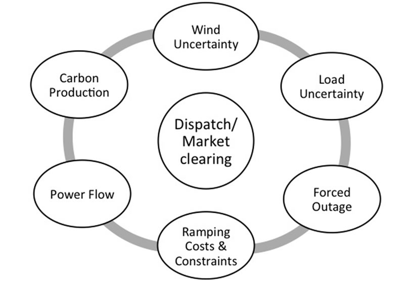
Figure 1. Sub-models within the Monte Carlo-Optimal Power Flow modeling framework.
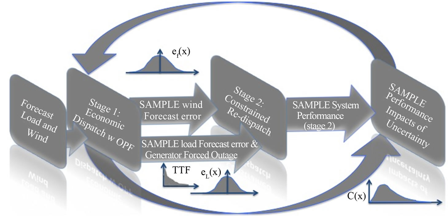
Figure 2. Conceptual diagram of Monte Carlo framework.
3.1. Wind Power Forecast Errors
The steps in developing a probability distribution of wind power forecast errors include 1) developing ten minute time series data for the power generation from each windfarm, 2) applying a basic forecasting algorithm to create both hour-ahead and ten-minute-ahead forecasts of wind power output, and 3) determining the distribution of the error in the forecast over the time horizon modeled.
For Step 1, the power generation from a wind farm is modeled using time series wind speed data that is translated to power output using a multi-turbine power curve algorithm. Ten-minute wind speed data from the National Renewable Energy Laboratory (NREL) study [8] and the GE 2.5 MW turbine power curve [9] are used to generate the output from the 5 hypothetical wind farms modeled for this study. The total windfarm output represents 10% (3 windfarms), 20% (4 windfarms) and 30% (5 windfarms) of the energy generation in the test system.
To capture the effect that geographic diversity has on decreasing the variability in wind power generation, the method presented in [10] was implemented. This algorithm involves adjusting single-point wind speed data with a moving block average to represent the wind speed across the wind farm. The turbine power curve is also adjusted as part of the algorithm in [10] to represent the effective aggregated power curve from the multiple turbines in the wind farm.
The adjusted wind speed data is translated to power output using the aggregated power curve. Figure 3 shows the original and adjusted wind power output, demonstrating the effect of geographic diversity in decreasing the variability of wind power generation. This figure shows the wind power output from a theoretical wind farm using the original windspeed data with the theoretical turbine power curve, as well as the adjusted wind speeds with the multi-turbine power curve representing a small wind farm of approximately 25 square kilometers.
Figure 4 depicts this data as a histogram of the frequency of power generated at each level. This figure demonstrates that for the data series that does not account for the geographic smoothing, the Original Data, there are many time periods with 0 MW generated from the wind farm. When the geographic smoothing is accounted for, there are almost no periods with 0 MW generated from the windfarm. This result is significant in that it highlights the fact that 0 MW output from large windfarms is relatively rare.
This histogram also demonstrates that there are fewer time periods with the maximum output once geographic smoothing is acknowledged. However, benefits from only rarely experiencing 0 MW are likely to outweigh any loss in revenue from the slight decrease in time periods with maximum output.
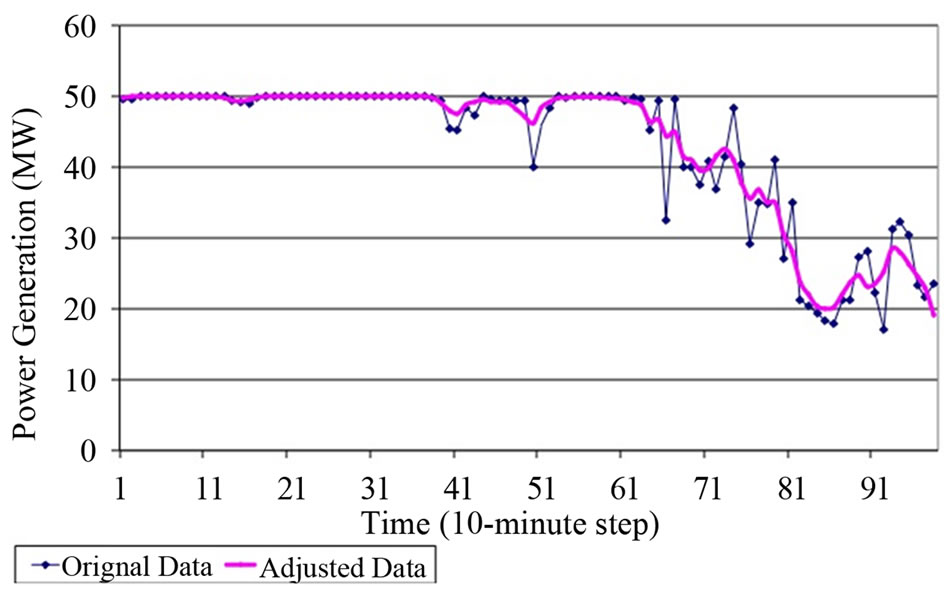
Figure 3. Windfarm power output, original and geographically smoothed using the multi-turbine power curve algorithm [10].
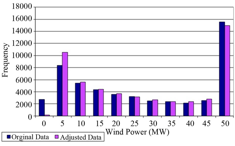
Figure 4. Distribution of wind power generation: unsmoothed and geographically smoothed.
This algorithm is applied to each individual windfarm. The additional smoothing effect, from having multiple windfarms that are geographically dispersed, is explicitly modeled through locating the windfarms at specific buses within the transmission test system [11].
Step 2 in developing the distribution of wind power forecast errors requires applying basic forecasting algorithms to create both hour-ahead and ten-minute-ahead forecasts. These different forecasts are used for the different stages within the larger two-stage optimization modeling and simulation framework (Section 2).
The forecasts at both hour-ahead and 10-minutes ahead are simple auto-regressive (AR) models with the appropriate lag. The AR model is used to forecast wind speed, and forecasted power generation is then determined from this forecasted wind speed data. Forecast error associated with these models are within acceptable accuracy bounds of wind forecasting literature [12].
In Step 3 the distribution of forecast errors is created by comparing the time series of forecasts to the time series of known wind power generation for different expected output levels. A sample set of the binned forecast errors is shown in Figure 5.
The data used for this analysis was obtained from NREL, with five clusters of locations within the New England region selected to represent the five windfarms modeled in this study. The locations are Manchester VT, Northfield MA, Nantucket MA, Orrington ME, and Pittsburg NH, using NREL locations [8]. Geographically these locations are proxies for Green Mountains Vermont, Central Massachusetts, Nantucket Sound, Off-shore Maine, and White Mountains New Hampshire. The resulting distribution of forecast errors for one of these locations is shown in Figure 5, and is representative of the distributions for all five modeled windfarm locations.
3.2. Electrical Demand Forecast Errors
Electrical demand data was obtained from the ISO New England archived load data [13]. An artificial neural network model was developed to forecast electrical load [14]. As with the distribution of wind forecast errors, a distribution of load forecast errors was created by comparing the time series of known load data to the time series of forecasted load data and recording the error in the forecast. The result of this analysis is shown in Figure 6.
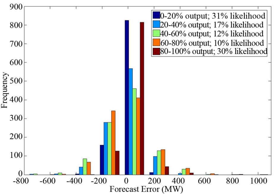
Figure 5. Error distribution for windfarm forecast.
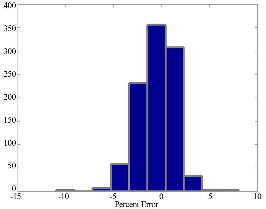
Figure 6. Error distribution for regional demand forecast.
3.3. Electrical Generator Forced Outage
In order to simulate realistic uncertainty in conventional generator reliability, a forced outage model was developed. The forced outage model is based on the traditional assumption of a negative exponential distribution of time to failure (TTF) [15]. Reliability of the generators are estimated by fuel type, based on information from the Generator Availability Database (GADS), and summarized in Table 1 [16].
Using these outage characteristics, random forced outages are sampled for each simulation in the two-stage optimization framework, and the available generation capacity is adjusted accordingly.
4. Electric Power System Model
The power system, including the high voltage transmission system, generator and load busses, is modeled with the IEEE 39 bus test system, which approximates a simplified version of the New England power system. The model is shown in Figure 7.
Power flow within the system is simulated with the MATPower ac power flow model [17] which determines the real and reactive power required to be generated by
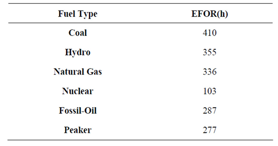
Table 1. Expected forced outage rates by fuel type, estimated from [16].
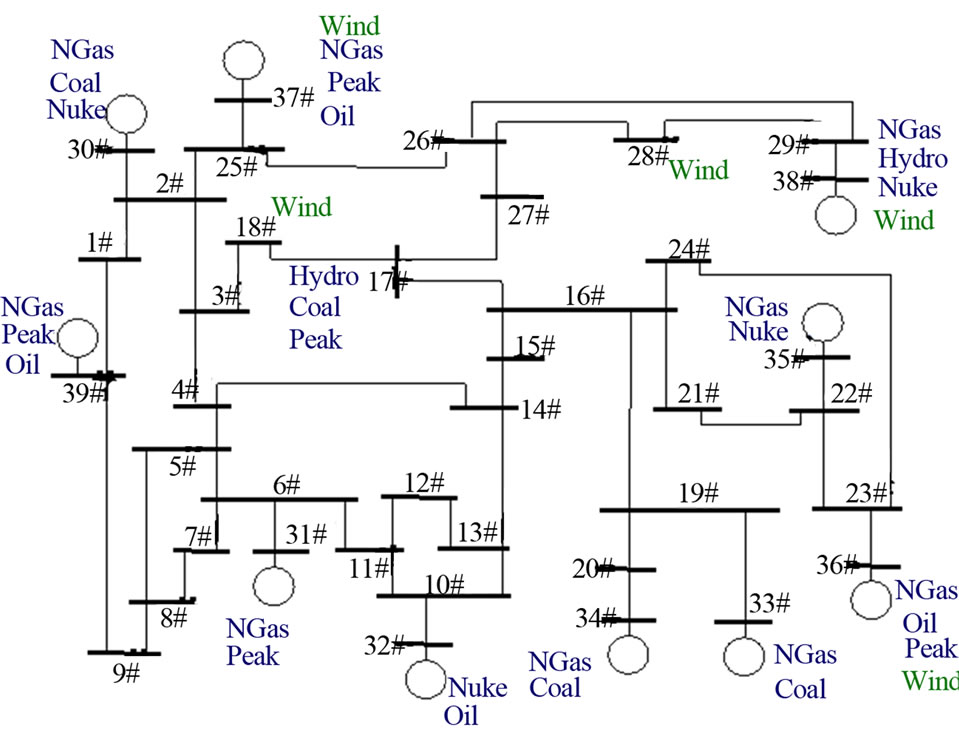
Figure 7. 39 Bus power system test system.
each generator in order to serve the given complex power demand, the power flow and losses on each transmission line, and the voltage phasor for each bus. This model is used for the stage 1 and stage 2 dispatch decision as shown in Figure 2.
4.1. Generation Technology Mix
As shown in Figure 7, the generating technologies included in the system model are steam turbines fueled by coal, fueled by oil, combined cycle plants fueled by natural gas (NGas), peaking plants fueled by natural gas (Peak), nuclear power generators, hydro-electric generators and wind power plants. Based on the historical technology mix for the New England region, the technology mix for the test system in Figure 7 is shown in Table 2.
The total generating capacity modeled in the test system represents approximately 14% of the total capacity in the New England region, based on the historical technology mix within the six New England states. “North” represents Maine, New Hampshire and Vermont, “Mass” is Massachusetts (the largest contributor to load and generating capacity in New England), and “South” represents Rhode Island and Connecticut.
One of the concerns over the increased use of wind power in the power system is the impact of the power variability, and uncertainty of that variability, on the other generators in the system. In order to maintain the instantaneous energy balance, other devices within the power system must ramp up if wind power suddenly drops off, and must ramp down if wind power generation increases. In order to accurately determine if the power system has adequate ramping capacity to mitigate this variability in the wind, the modeling framework developed here constrains the response of each generator to a wind or load forecast error, or generator outage, to be within its actual ramping capability [18-23]. This ramping capability is shown in Table 3. The implementation of the ramping constraints is within the modeling framework discussed in Section 2.
The final element in fully modeling generator ramping is to include the cost to the generators, which includes the operation and maintenance costs from the increased cycling [18-20]. These costs are shown in Table 4. This table also shows the fixed and variable operating and
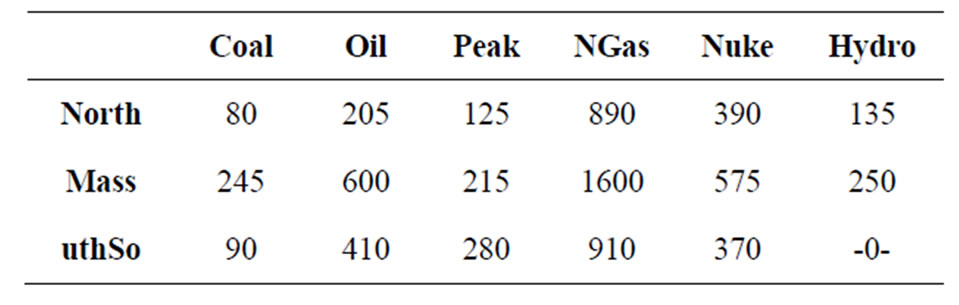
Table 2. Generator technology mix for IEEE 39 bus test system, (MW).
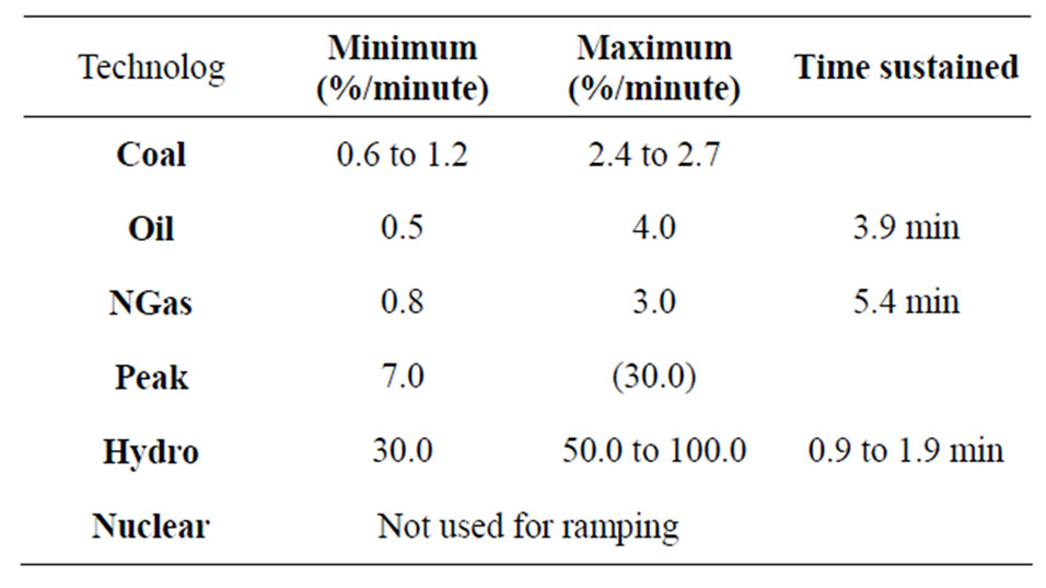
Table 3. Generator Ramping, showing minimum and maximum ramping rates as percent of capacity per minute, and maximum duration, or time sustained, for the ramping period.
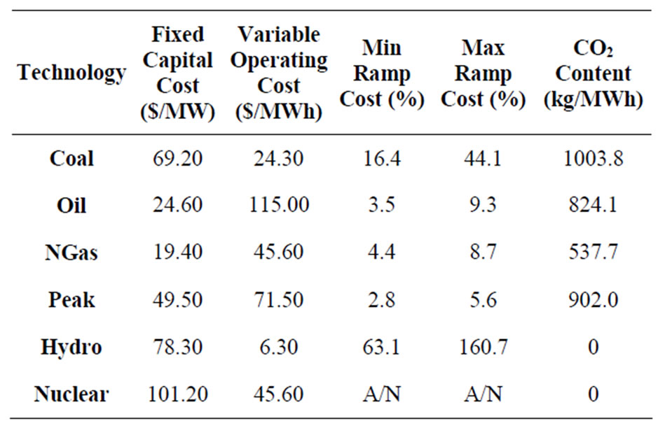
Table 4. Generator costs and fuel carbon content. Ramping costs are shown as a percent increase to the variable operating cost.
maintenance costs for each generator technology category.
4.2. Generator Carbon Dioxide Emissions
The calculation for carbon dioxide, CO2, emissions from the electricity generation in the test system relies on information from the US Environmental Protection Agency, EPA [24,25]. The expression used is
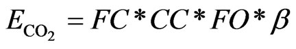 (1)
(1)
where  is kg of CO2 emissions, FC is the fuel combusted, CC is the carbon content coefficient of the fuel, FO is the fraction of carbon oxidized and β is the ratio of the molecular weight of carbon dioxide to carbon [24].
In applying Equation (1), the fuel combusted is obtained from the estimated heat rate of each generating unit and the output of that unit as determined by the Matpower optimal power flow, OPF. The heat rate data are from EPA and FERC (Federal Energy Regulatory Commission) filings by utility companies. The heat rate and capacity factor for every generating unit in New England were used to determine an average regional heat rate for each generating technology. The coefficient of carbon content is obtained from the EPA [24,25]. For this study it is assumed that 100% of the carbon is oxidized, and  [24]. The product of the average regional heat rate, the carbon content coefficient and the molecular conversion to CO2 is shown in the far right column of Table 4.
5. Analysis of Responsive Demand
The fundamental objective of the electric power system is to supply all electrical demand, at least cost, while maintaining reliability and stability. Implicit in this objective is the assumption that electrical demand at each moment is exogenous to the system operations, and thus generators, transformers, and other devices under control of the system operators must be operated in a manner that will provide all the demanded electrical use.
This historical paradigm is changing with the introduction of variable energy resources (VER) such as wind and solar power, along with smart grid technologies that facilitate greater active involvement of demand in power system operations. Rather than strictly relying upon conventional generating technologies to mitigate the variable output of VER, power system operators are looking into using responsive demand, as well as storage, to be part of maintaining the system energy balance [26].
The analysis presented here incorporates responsive demand in two ways. First, all load is assumed to have flexibility in the amount of electricity actually demanded. This is implemented through a demand cost curve for which the final 10% - 15% of MW demanded can be not served (or interrupted) in real-time by the system operator at a cost of $100/MWh [13]. In the absence of this flexibility, the cost to reduce demand is set to $10,000/ MWh. The OPF algorithm will decide to pay load to not consume, rather that pay generators to generate, if this is the least cost, or only, option to mitigate the forecast errors from wind, load, or a generator outage.
The second option for including demand response in the modeling framework is to identify resources that would be willing to either cut or shift their demand in advance of real time [26-28]. For this modeling framework, demand response can be implemented both in the hour-ahead and ten-minute ahead dispatch, or market stages. In this option, the regional demand is decreased proportionally by the amount of forecast error that will be mitigated. For the simulations presented here, 50% of the expected forecast error is mitigated with responsive demand at each market stage, when demand response is used.
6. Results and Discussion
The modeling framework defined in Section 2 is used with the 39 bus test system and input data as defined in Sections 3, 4 and 5. For running the simulations, a set of base case scenarios is defined. Each of these base case scenarios is implemented in a Monte Carlo framework, with sampled values for uncertain inputs as previously defined. The characteristics of the resulting system parameters (locational marginal price, CO2 emissions, wind power used, and production costs) are then estimated and the system impact of uncertainty analyzed.
6.1. Scenario Definition
A set of base case scenarios, shown in Table 5, define the system configurations simulated and analyzed in this study. As this table shows, scenarios are identified according to the wind penetration by energy, as well as a high, medium, or low forecast level for each wind farm.
The expected output for each forecast level is defined in terms of the actual wind data and 10-minute time series wind generation from each windfarm. From this data a low forecast expected value is an output level of 11% of installed windfarm capacity, medium forecast is 44% of installed capacity and high forecast expected output is 87% of the installed windfarm capacity. With all permutations of high-medium-low forecast levels at each windfarm modeled, the result is 27 permutations at 10% wind penetration (three windfarms), 81 permutations at 20% wind (four windfarms), and 243 permutations at 30% wind penetration (five windfarms).
There are three load levels, high medium and low, defined in terms of the reserve margin, or percent of generating capacity above the peak load level. Finally, demand response can be included as 15% real-time responsive demand, and the hour-ahead/10-minute-ahead demand advance demand response.
This results in a total of 8424 base case scenarios. With 200 draws for the Monte Carlo simulations, this leads to more than 1.6 million total simulations to be used for analyzing the impact of uncertain system inputs on power system performance.
6.2. Generator Dispatch by Fuel Type
In the system without any wind installed, averaged across
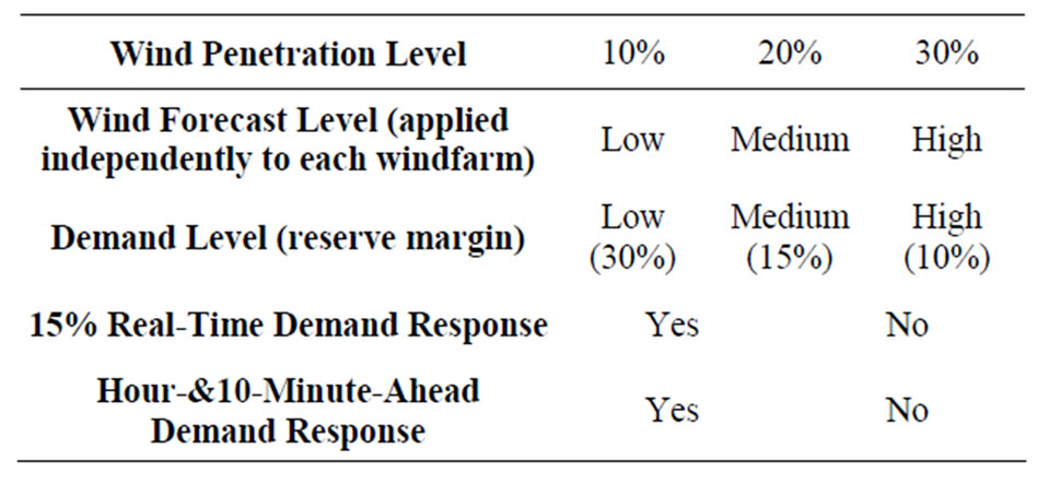
Table 5. Base case scenario identification.
the three load levels and the results from load forecast and forced outage uncertainties, the system is dispatched as shown in Figure 8. This figure shows that natural gas combined-cycle plants account for approximately 50% of the energy use, and also that the peaking units are used to supply 6% of the energy.
Figures 9-11 show the generator dispatch mix with 10%, 20% and 30% of energy from wind power, respectively. An initial observation for these figures is that the wind power actually accounts for more than the targeted amount, demonstrating a higher capacity factor than anticipated in the NREL dataset [29]. It is also apparent that the natural gas fired plants, both combined cycle and peaking combustion turbines, are the units most directly affected by the integration of wind power. The combined cycle plant contribution decreases from 52% with no wind to 21% with 30% wind. The peaking units are also used to supply less total energy, decreasing from 6% with no wind installed, to 1% at 30% wind penetration. It is also interesting to note that at lower wind penetrations the use of peaking units is even less, accounting for less than 1% of the total energy supplied. These values do not capture the increase in the variability, or cycling, of these units, which does increase with increased wind penetration.
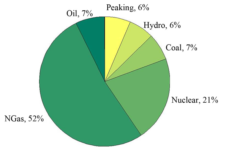
Figure 8. Generator dispatch by fuel type—no wind.
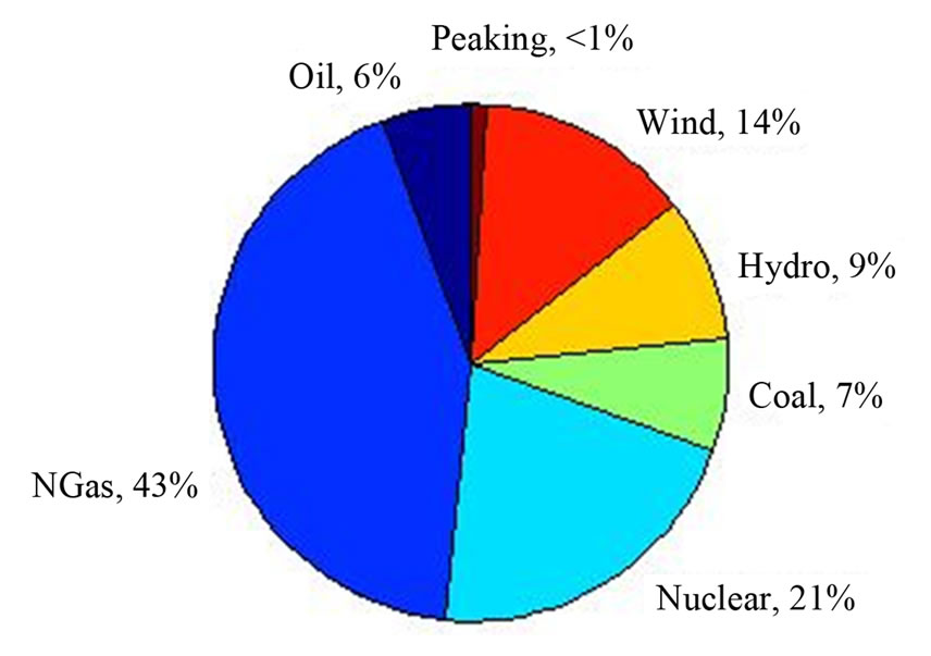
Figure 9. Generator dispatch by fuel type—10% wind penetration.
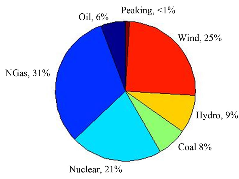
Figure 10. Generator dispatch by fuel type—20% wind penetration.
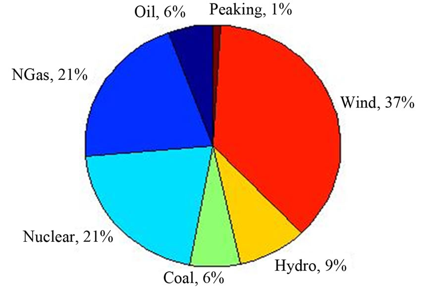
Figure 11. Generator dispatch by fuel type—30% wind penetration.
6.3. Carbon Dioxide Emissions
With the decreased reliance upon fossil fuels, the total carbon dioxide emissions for the test system decrease also. Figures 12-15 show the distributions of carbon dioxide emissions for no wind, 10%, 20% and 30% wind penetration scenarios respectively.
The no wind scenarios show that the total CO2 emissions ranges between approximately 3000 and 4500 tons of CO2 for the test system. Figures 13-15 show not only a decrease in the maximum amount of CO2 emissions, for the high load cases, but also a lowering of the minimum amount of CO2 emissions possible across all scenarios, reaching as low as 750 tons for almost 30% of the low load cases with 30% wind, a decrease of almost 75% in emissions.
This significant decrease in CO2 emissions across all scenarios is one of the anticipated benefits of greater wind power integration, and is demonstrated to be achieved in these simulations.
6.4. Electricity Price
The electricity price, calculated as the Lagrangian multiplier, λ, from the energy balance constraint in the optimal
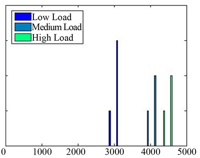
Figure 12. CO2 emissions (tons) with no wind.
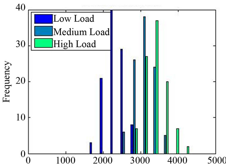
Figure 13. CO2 emissions (tons) with 10% wind.
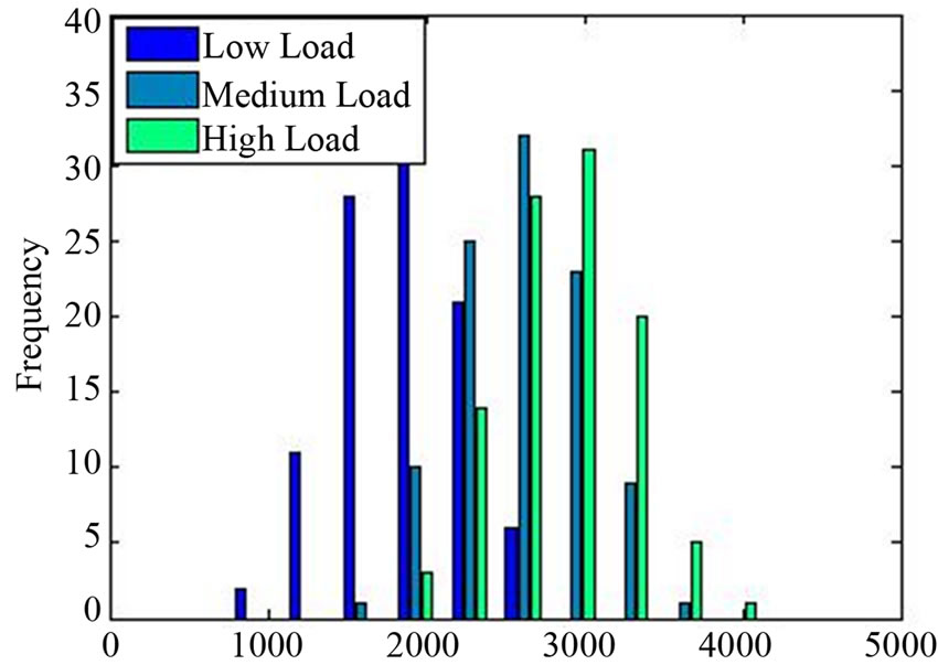
Figure 14. CO2 emissions (tons) with 20% wind.
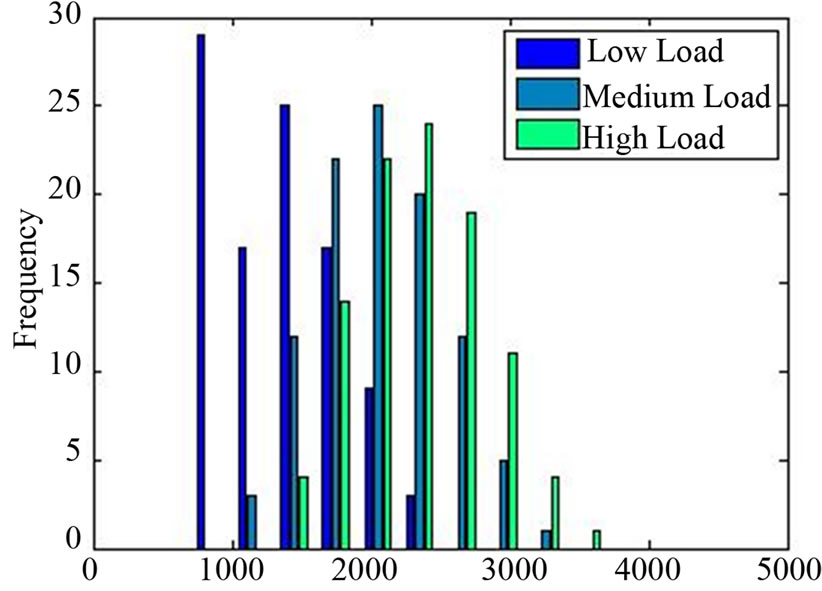
Figure 15. CO2 emissions (tons) with 30% wind.
power flow, is referred to as the locational marginal price, LMP. With no wind installed in the system, this value ranges between $45/MWh and $120/MWh, with a slight decrease in both value and variability as demand response is introduced. A summary of LMP and its variability, measured as the standard deviation, is shown in Table 6.
Figure 16 shows a bimodal distribution for the LMP, typical for the simulations within the modeling framework defined here. The lower range of electricity prices are in the same range as occurs when no wind is installed in the system. As wind power is introduced however, the system is less able to respond to all the uncertainties— wind forecast errors, load forecast errors and generator forced outages. With ramping constraints imposed on the conventional generators, such that each unit can only ramp up or down within its technical capability in response to the uncertainties, there are scenarios encountered by the Monte Carlo simulations in which the system must interrupt load beyond that which is made available (if any) through demand response programs. In these situations, the system is required to pay that load $10,000/MWh for each MW unserved.
These events, leading to price spikes, are seen in Figure 16 in the rightmost bars clustered at $10,000/MWh. The number of these price spike events does increase significantly when wind power is installed, as comparedto the system with no wind, Table 6. Moderate
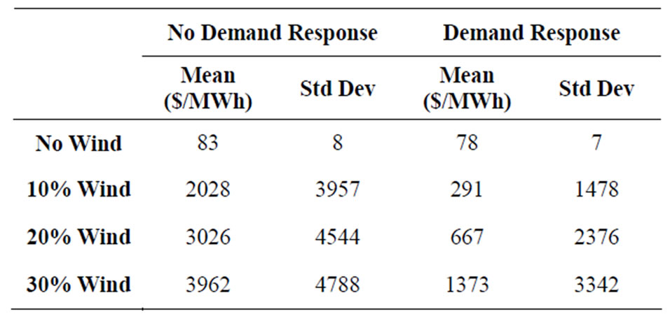
Table 6. Impact of increasing wind penetration on electricity price, LMP, with and without demand response, across all load levels.
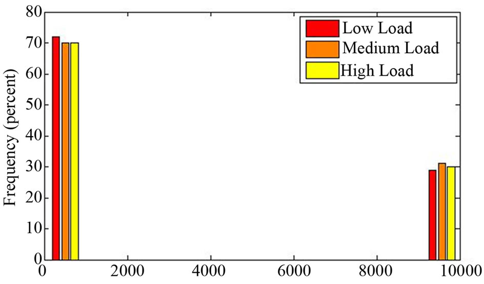
Figure 16. LMP for 20% wind with no demand response ($/MWh).
introduction of demand response decreases the number of these events significantly though, as seen by comparing the two rightmost columns for “Demand Response” in Table 6 to those for “No Demand Response”. Looking at the medium wind penetration of 20% for example, the introduction of demand response decreases the number of price spike events from 30% of the scenarios to 6%. Additional demand response resources or other options for flexible system response could be used to reduce and even eliminate these price spikes. Such measures are being investigated within this modeling framework and by many other researchers, but are beyond the scope of the analysis for this paper.
6.5. Wind Used & Wind Spilled
With the fuel source for wind generation being free, there is an expectation that all wind power generation made available to the system could be used to serve load. In order to maintain the system reliability, however, so that supply is equal to demand at all times, it can be necessary to not use, or spill, some available wind power.
At the 10% wind penetration level, there is almost no need to spill wind power—for almost all scenarios with wind forecast uncertainty, load uncertainty and generatior forced outages—the system is able to utilize all available wind power and serve load. With 20% wind, and particularly at low load levels, the system needs to spill a relatively low amount of wind power, averaging 3 MW of wind across all scenarios. In very few scenarios, 75 MW to 125 MW of wind power is spilled, in order to maintain the system energy balance (out of 4000 MW wind power installed for 20% wind penetration).
At 30% wind penetration, there is still relatively little need for the system to spill wind power, with an average across all scenarios around 14 MW. Figure 17 shows the distribution of MW wind power spilled for the scenarios with 30% wind penetration (6400 MW installed wind capacity) and no demand response. The leftmost cluster of bars shows that the majority of scenarios do not require spilling any wind. However, with other uncertainty in the system, and the conventional generator response to shortfalls and over-generation constrained within its ramping limits, there are a number of scenarios in which the system is required to spill wind power in order to maintain the energy balance.
7. Conclusions
Globally, power systems are expected to be integrating continually increasing amounts of wind power. The uncertainty and variability of this resource requires new analysis and operating methods in order to ensure power system stability and reliability. This paper has presented an analysis of integrating up to 30% wind power into a
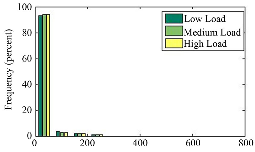
Figure 17. Wind spilled for 30% wind with no demand response.
power system, using the IEEE 39 bus test system and input data representing the New England region. The results show that the system is able to maintain reliability, in terms of meeting the energy balance constraint, at all levels of modeled wind penetration, including the high level of 30% (by energy) wind penetration.
Though incorporating wind power generation into the electric power system introduces a significant new source of variability and uncertainty, it is not the only resource with these properties. With the growing concern around the impacts of wind uncertainty, it is important to consider all sources of uncertainty in the system in order to fully model the results of stochastic behavior. Conventional generators experience forced outages and the system will experience load forecast errors along with the wind forecast errors. All three of these sources of uncertainty are quantified, modeled and analyzed in this paper.
A second feature of wind power, as the turbines are aggregated in wind farms, is the potential for the geographic smoothing, or decrease in variability, of the aggregated output as compared to the power output from a single wind turbine. This property has also been modeled in the analysis presented here, with the geographically smoothed wind power generation used as input into the simulations. These results demonstrated a significant decrease in time steps with 0MW of wind generation from the aggregated output of a windfarm, as compared to the higher likelihood of 0MW being generated from a single wind turbine.
For simulation results, the IEEE 39 bus test system is modeled with 10%, 20% and 30% wind penetration. The results indicate that the inclusion of wind generation, in particular at high penetration levels, has a significant positive impact on decreasing carbon dioxide emissions: up to 75% reduction at 30% wind, over the no-wind case. This is primarily due to the displacement of natural gas fired generation by wind. The anticipated benefit of reduced CO2 emissions is achieved as a result of this decreased fossil fuel use.
There are also challenges that result: price spikes occur, specifically due to the need for down ramping of expensive demand. However, the inclusion of demand response resources shows significant potential in mitigating the challenges associated with high wind penetration. At higher levels of wind penetration of 20% and 30%, and no additional mitigating options, price spikes can occur up to 30% of the time steps. With no additional system flexibility for responding to the wind, load and generator availability uncertainty, this high number of price spike events could decrease the value of the other benefits from including wind power. However, with inclusion of even moderate demand response levels, the number of price spike events is significantly reduced. These results are shown in Table 6 in terms of the mean and standard deviation of the electricity price in the different wind penetration scenarios, with and without demand response.
Ongoing work with the modeling framework presented here includes investigation into additional system flexible resources such as the use of storage facilities, optimizing demand response resource use and developing a methodology for flexible wind dispatching.
8. Acknowledgements
This work was funded by the US Department of Energy in cooperation with the Consortium for Electric Reliability Technology Solutions (CERTS), PSERCs industry members (Power Systems Engineering Research Center), and NSF PIRE and SEP programs, grant numbers OISE 1243482 and 1230913.
REFERENCES
- G. Hinkle, R. Piwko, J. Norden, B. Henson, G. Jordan, A. Chanal, N. Miller, S. Meeran, R. Zavadil, J. King, T. Mousseau and J. Manobianco, “New England Wind Integration Study,” ISO New England, Holyoke, 2010.
- New York Independent System Operator, “Growing Wind: Final Report of the NYISO 2010 Wind Integration Study,” 2010.
- R. Doherty, L. Bryans, P. Gardner and M. O’Malley, “Wind Penetration Studies on the Island of Ireland,” Wind Engineering, Vol. 28, No. 1, 2004, pp. 27-41. http://dx.doi.org/10.1260/0309524041210856
- H. K. Jacobsen and E. Zvingilaite, “Reducing the Market Impact of Large Shares of Intermittent Energy in Denmark,” Energy Policy, Vol. 38, No. 7, 2010, pp. 3403- 3413. http://dx.doi.org/10.1016/j.enpol.2010.02.014
- EnerNex Corporation, windLogics, Midwest ISO, Minnesota Public Utilities Commission, “2006 Minnesota Wind Integration Study Volume I,” Midwest ISO, Carmel, 2006.
- Y.-H. Wan, “Analysis of Wind Power Ramping Behavior in ERCOT,” National Renewable Energy Laboratory, Golden, Lakewood, 2011.
- BENTEK Energy, LLC, “How Less Became More: Wind, Power and Unintended Consequences in the Colorado Energy Market,” Independent Petroleum Association of Mountain States, Washington DC, 2010. http://www.ipaa.org/about-ipaa/
- M. Brower, “Development of Eastern Regional Wind Resource and Wind Plant Output Datasets: March 3, 2008-March 31, 2010,” National Renewable Energy Laboratory, Golden, Lakewood, 2009.
- GE Wind, “Wind Turbines—Wind Power | GE Energy,” 2013. http://www.ge-energy.com/products_and_services/products/wind_turbines/index.jsp
- P. Norgaard and H. Holttinen, “A Multi-Turbine Power Curve Approach,” Proceedings of Nordic Wind Power Conference, Gothenburg, 1-2 March 2004, pp. 1-5.
- J. B. Cardell and C. L. Anderson, “Analysis of the System Costs of Wind Variability through Monte Carlo Simulation,” Proceedings of the 43rd Hawaii International Conference on System Sciences, Honolulu, 5-8 January 2010, pp. 1-8.
- B.-M. Hodge and M. Milligan, “Wind Power Forecasting Error Distributions over Multiple Timescales,” IEEE Power and Energy Society General Meeting, Detroit, 24- 29 July 2011, pp. 1-8.
- ISO New England, “ISO New England - ISO New England Inc.,” 2013. http://www.iso-ne.com/
- C. Y. Tee, J. B. Cardell and G. W. Ellis, “Short-Term Load Forecasting Using Artificial Neural Networks,” Transactions on Power Systems, Vol. 7, No. 1, 2009, pp. 124-132.
- J. D. Hall, R. J. Ringlee and A. J. Wood, “Frequency and Duration Methods for Power System Reliability Calculations: I-Generation System Model,” IEEE Transactions on Power Apparatus and Systems, Vol. PSA-87, No. 9, 1968, pp. 1787-1796.
- North American Electric Reliability Corporation, “Generating Availability Data System (GADS),” 2013. http://www.nerc.com/pa/RAPA/gads/Pages/default.aspx
- R. D. Zimmerman, “Matpower 4.0b4 User’s Manual,” 2010, pp. 1-105. http://www.pserc.cornell.edu/matpower/
- C. W. Hamal and A. Sharma, “Adopting a Ramp Charge to Improve Performance of the Ontario Market,” The Association of Power Producers of Ontario, Toronto, 2006.
- C. Wang and S. M. Shahidehpour, “Optimal Generation Scheduling with Ramping Costs,” IEEE Transactions on Power Systems, Vol. 10, No. 1, 1993, pp. 11-17.
- G. B. Shrestha, K. Song and L. Goel, “Strategic SelfDispatch Considering Ramping Costs in Deregulated Power Markets,” IEEE Transactions on Power Systems, Vol. 19, No. 3, 2004, pp. 1575-1581. http://dx.doi.org/10.1109/TPWRS.2004.825891
- G. Lalor and M. O’Malley, “Frequency Control on an Island Power System with Increasing Proportions of Combined Cycle Gas Turbines,” 2003 IEEE Bologna Power Tech Conference Proceedings Vol. 4, Bologna, 23-26 June 2003, p. 7.
- Northeast Power Planning Council, “Natural Gas Combined-Cycle Gas Turbine Power Plants,” Northwest Power and Conservation Council, Portland, 2002. http://www.westgov.org/wieb/electric/Transmission%20Protocol/SSG-WI/pnw_5pp_02.pdf
- J. Lindsay and K. Dragoon, “RNP Summary Report on Coal Plant Dynamic Performance Capability,” Renewable Northwest Project, Portland, 2010.
- US Environmental Protection Agency, “US Inventory of Greenhouse Gas Emissions and Sinks, Fast Facts, Reference Tables and Conversions,” EPA 430-R-13-001, 2013. http://epa.gov/climatechange/Downloads/ghgemissions/fastfacts.pdf
- US Environmental Protection Agency, “Inventory of U.S. Greenhouse Gas Emissions and Sinks: 1990-2011,” EPA 430-R-13-001, US Environmental Protection Agency, 2013.
- P. Cappers, A. Mills, C. Goldman, R. Wiser and J. H. Eto, “Mass Market Demand Response and Variable Generation Integration Issues: A Scoping Study,” 2011. http://epa.gov/climatechange/Downloads/ghgemissions/fastfacts.pdf
- M. Klobasa, “Analysis of Demand Response and Wind Integration in Germany’s Electricity Market,” IET Renewable Power Generation, Vol. 4, No. 1, 2010, p. 55. http://dx.doi.org/10.1049/iet-rpg.2008.0086
- B. Perlstein, L. Battenberg, E. Gilbert, R. Maslowski, F. Stern, S. Schare, K. Corfee and R. Firestone, “Potential Role of Demand Response Resources in Maintaining Grid Stability and Integrating Variable Renewable Energy under California’s 33 Percent Renewable Portfolio Standard,” California’s Demand Response Measurement and Evaluation Committee, Navigant Consulting, Inc., Chicago, 2012.
- National Renewable Energy Laboratory (US), “Wind Systems Integration—Eastern Wind Integration and Transmission Study,” 2010. http://www.nrel.gov/wind/systemsintegration/ewits.html