Engineering
Vol. 2 No. 10 (2010) , Article ID: 3180 , 11 pages DOI:10.4236/eng.2010.210103
Using Image Analysis for Structural and Mechanical Characterization of Nanoclay Reinforced Polypropylene Composites
Composites Research Group Department of Mechanical Engineering Durban University of Technology, Durban – South Africa
E-mail: kannyk@dut.ac.za
Received July 9, 2010; revised September 1, 2010; accepted September 8, 2010
Keywords: Polymer Clay Nanocomposites, Transmission Electron Microscope, Optical Microscope, Intercalation/Exfoliation, Micromechanical Modeling
ABSTRACT
This paper focuses on the micromechanical study of the tensile property of Polymer-Clay Nanocomposites (PCN). Polypropylene (PP) filled with nanoclay is chosen as the PCN. Measurements of optical dispersion parameters (as discussed by Basu et al., namely, exfoliation number (ξn), degree of dispersions (c) and agglomerate %) in PCN system were carried out using Transmission Electron Microscopy (TEM) and Optical Microscopy (OM). The experimentally obtained tensile modulus is compared with theoretically obtained modulus values from the optical dispersion parameters and observed a close matching between these values. Also, the tensile values are compared with other standard theoretical models and observed that the results obtained from optical dispersion parameters are suited well with experimental results.
1. Introduction
Polymer filled with nanolayered silicate clay has become a significant research interest in recent past and continues to be an area of important focus because they exhibit dramatic improvement in properties at very low clay filler contents. Usually micron-Scale conventional fillers are added in polymer in the form of particles or fibres shaped additives. However, the addition of these particles in polymer imparts increased weight, brittleness, opacity etc. A polymer nanocomposite (in which at least one dimensions of reinforcement material in nanometer level ~100 nm) on the other hand provides enhanced property benefits to polymer system at very low weight concentration level (~3 to 5 wt.%). Commonly used nanoparticles in polymer matrix are nanolayered clays, because of their ease availability and cost effectiveness [1-3].
The addition of nanoclay in polymer matrix result in the formation of two types of nanocomposites structures, namely, an intercalated or an exfoliated structure. The host polymer matrix enters into the interlayer spacing of nanoclay and increases the interlayer of clay more and maintains the parallel arrangement of nanolayers of clay in matrix and this structure is called an intercalated structure. If the nanolayers of clays are randomly dispersed in matrix, then the structure is called an exfoliated structure. These intercalated and exfoliated structures can be examined by using TEM and X-ray diffraction (XRD) methods. In general, exfoliated structure provides improved properties than intercalated nanocomposite structure due to increase of net aspect ratio of clay nanolayers (length/thickness). However, if the concentration of clay is increased, the composite structure becomes intercalated structures and also some times leads to improved properties which are primarily due to the major contribution of clay property rather than nanoclay composite structure (exfoliated) [4-7]. Each nanolayer of clay constitute of elliptical disc like platelet shaped structure, of length and width varying from 100 nm to 2000 nm and thickness of about 1 nm.
It is well known fact that the property of PCN depends on degree of dispersions of clays. The properties are good if the dispersion of clays are proper and with no agglomeration [8-11]. This phenomenon suggests that there exists a link between dispersions and the property of composites. The better the dispersion of nanolayers in polymer, better property enhancements can be obtained. However, the nanolayers are not easily dispersed in most polymers due to their preferred face-to-face stacking of clay platelets in agglomerated tactoids. Studying the characteristics of dispersions of particles (distribution, arrangement, orientation, etc) helps to understand the property of composites in better way. Basu et al. [12] has done image analysis using sterelogy of TEM and Optical Microscope (OM) pictures and studied the extent of dispersion of particles using dispersion parameters (namely: exfoliation number, interparticle distance and agglomeration %). In this work, we used these optical dispersion parameters and further extended these parameters to study the tensile property of composites. PCN system chosen in this study was polypropylene (PP) as matrix polymer material and reinforcement as nanoclay particles. The objective of this work is to measure the tensile modulus using optical dispersion parameters. The theoretically measured tensile modulus using optical dispersion parameters is then compared with experimentally obtained results and also with various standard micromechanical models. It is observed that the theoretical results measured using this optical dispersion parameters correlated well with that of experimental results than other standard models. The out come of the results are discussed in this paper.
2. Experiments
2.1. Materials and Manufacturing
Cloisite 15A is a natural montmorillonite organically modified with a quaternary ammonium salt and was obtained from Southern Clay Products, USA. Polypropylene pellets were procured from Chempro, South Africa.
The nanocomposite panel was manufactured using a melt-blend technique. In this technique, the polypropylene pellets and the nanoclay were combined in a REIFFENHAEUSER screw extruder. The extruder has a 40 mm diameter single rotating screw with a length/diameter ratio (L/D) of 24 and driven by a 7.5 kW motor. Three heating zones along the length of the screw were set up to gradually heat the pellet/clay mixture. The temperatures in these zones were as follows: Zone 1 (pellet loading end) was set at 170˚C, Zone 2 (centre region of screw) was at 190˚C, and Zone 3 (extrusion end) was maintained at 210˚C. This temperature gradient setup was created to avoid thermal shock, (i.e., the heating condition is fixed up in such a way that the melt polymer samples exhibits uniform gradient of temperature across the length of extrusion unit instead of sudden change of temperature).
2.2. Characterization
Microscopic investigation of selected nanocomposite specimens at the various weight compositions were conducted using a Philips CM120 BioTWIN transmission electron microscope with a 20 to 120 kV operating voltage. The cryo and low dose imaging TEM has BioTWIN objective lens that gives high contrast and a resolution of 0.34 nm. The specimens were prepared using a LKB /Wallac Type 8801 Ultramicrotome with Ultratome III 8802A Control Unit. Ultra thin transverse sections, approximately 80-100 nm in thickness were sliced at room temperature using a diamond coated blade. The sections were supported by 100 copper mesh grids.
3 cm × 3 cm × 3 mm specimen of PP-clay series were taken and cut into two across the mid portion of the specimen. The cut portion is viewed through optical microscope at 100x using ZEISS AXIO LAB optical microscope. Tensile tests were performed on virgin PP and the nanocomposite specimens using the LLOYDS Tensile Tester fitted with a 20 kN load cell. The tensile tests were performed at a crosshead speed of 1 mm/min in accordance with the ASTM D3039 standard.
3. Results and Discussions
3.1. Rules of Mixture and Halpin-Tsai Formulation
The parallel model (rules of mixture) has been applied for the prediction of Young’s modulus and is given the Equation (1). Young’s modulus of clay and PP are taken as 167 GPa and 1 GPa respectively.
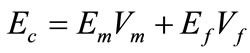 (1)
(1)
Figure 1 shows the experimental and rules of mixture values. There is a large variation in experimental and theoretical values. Equation (1) shows that the theory does not account for the aspect ratio and the shape of the fillers.
This theory is further improved by Halpin Tsai [13] which predicts the stiffness of particulate filled composites as a function of aspect ratio. The longitudinal and transverse moduli E11 and E22 are expressed in the general form as per Equation (2).
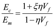 (2)
(2)
Further  is given by
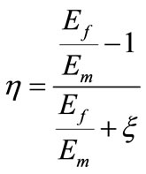 (3)
(3)
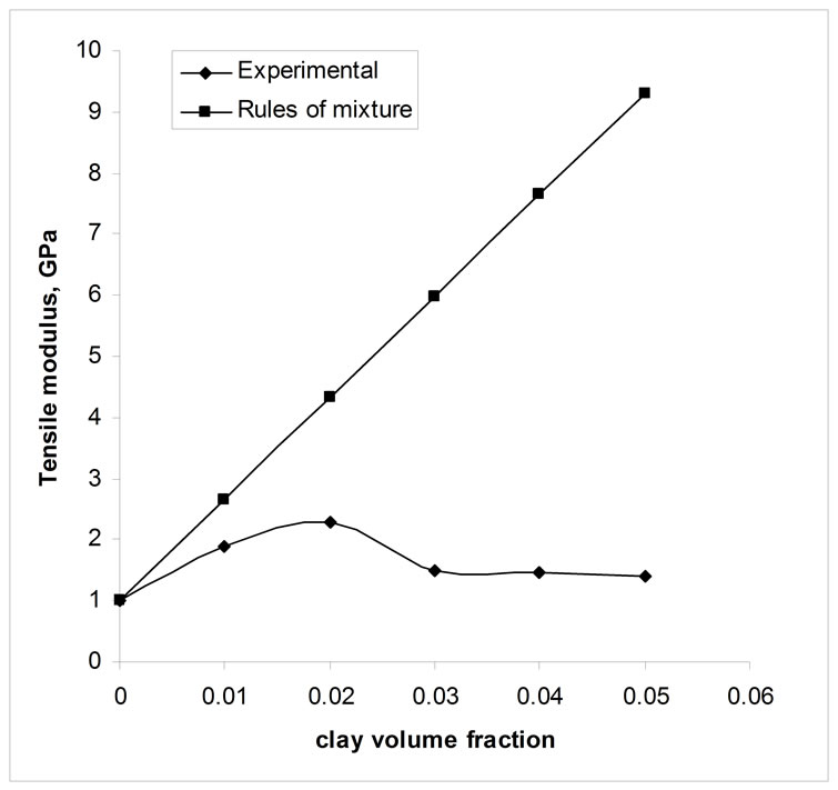
Figure 1. Comparison of Rules of mixture and experimental results.
 = 2 (a/b) in which ‘a’ and ‘b’ are the length and thickness of the fibre. The effect of ‘a’ on modulus of composites is shown in Figure 2. At higher clay content, there is a large variation in experimental and theoretical results. The existence of agglomeration, intercalated structures, etc, of clay particles in matrix polymer might have reduced composite properties along the loading direction and this leads to the low modulus value than the theoretical values.
3.2. Stack Model
The polymer-clay nanocomposites consist of clay platelet reinforcement in variety of polymer matrices for the formation of either intercalated or exfoliated structure. However, in most cases exfoliation is thermodynamically unfavourable and most process techniques lead only to intercalated structures particularly at higher clay content [8-11]. Here an attempt is made to understand the influences of incomplete exfoliation on nanocomposite stiffness using composite theory. For this analysis, the stacking of clay platelets within a particle is treated in a very simple fashion, i.e. platelets of equal diameter are stacked directly one over the other and the load is applied parallel to the platelet edges, as shown in Figure 3. Matrix polymer is assumed to be present in the interlayer region of two clay nano platelets (layers).
The tensile modulus of a simple stack in the direction parallel to its platelets can be estimated by using the rule of mixture, as suggested elsewhere [14]. Stack modulus can be found out from rules of mixture as per Equation (4).
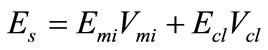 (4)
(4)
The stack modulus (Es) obtained from Equation (4) is substituted in Equation (1) in place of Ef. The matrix thickness in the stacks plays a significant role in the composite modulus. If matrix thickness in the clay interlayer region is more, then the effective clay volume fraction will reduce. Figure 4 shows the effect of matrix thickness in interlayer region and their corresponding decrease in the clay volume fraction. Also, at given matrix thickness, the volume fraction of clay stack remains constant irrespective of number of stacks.
Figure 5 show the comparison of experimental results with the theoretical values of stack model. It is observed that matching is good at clays volume fraction of 0.02 and 0.03, however at higher clay content the deviations is more. By altering stack thickness and thickness of matrix at interlayer (dms), some matching can be expected. Even though at higher clay content, the structure becomes intercalated structure (stacking sequence), the theoretical and experimental results have not matched well. Possibly other factors like aspect ratio, interface property etc, could have influenced the experimental results.
3.3. Mori-Tanaka Theory
Mori-Tanaka micromechanical model have been proposed to predict the elastic constants of discontinuous fibre/flake composites [15]. This model depends on parameters including particle/matrix stiffness ratio; particle
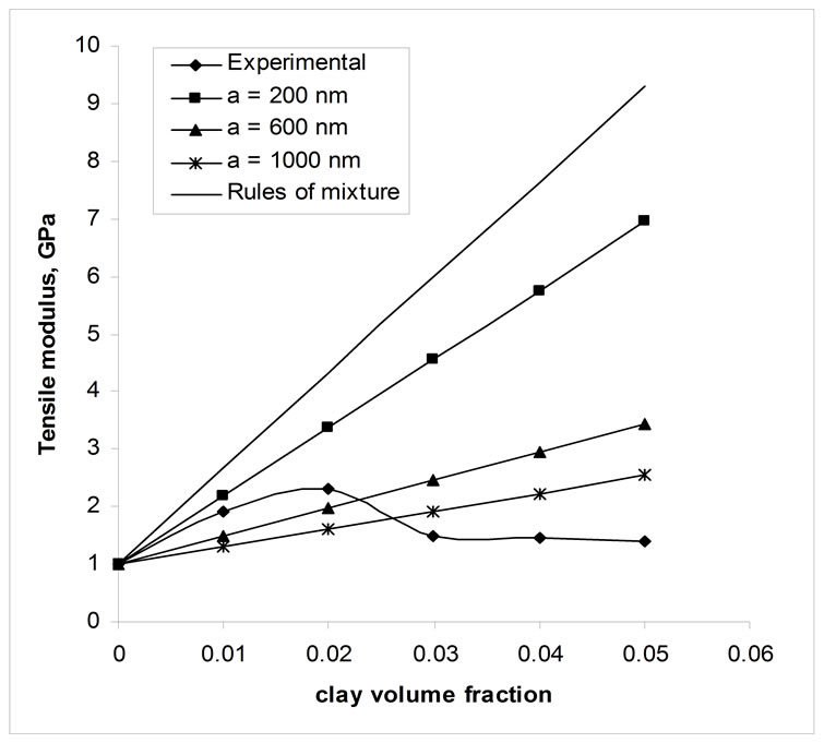
Figure 2. Comparison of Halpin-Tsai theory and experimental results.

Figure 3. Tensile loading in stack model.
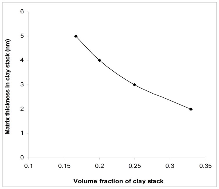
Figure 4. Effect of matrix thickness in clay nanolayer.
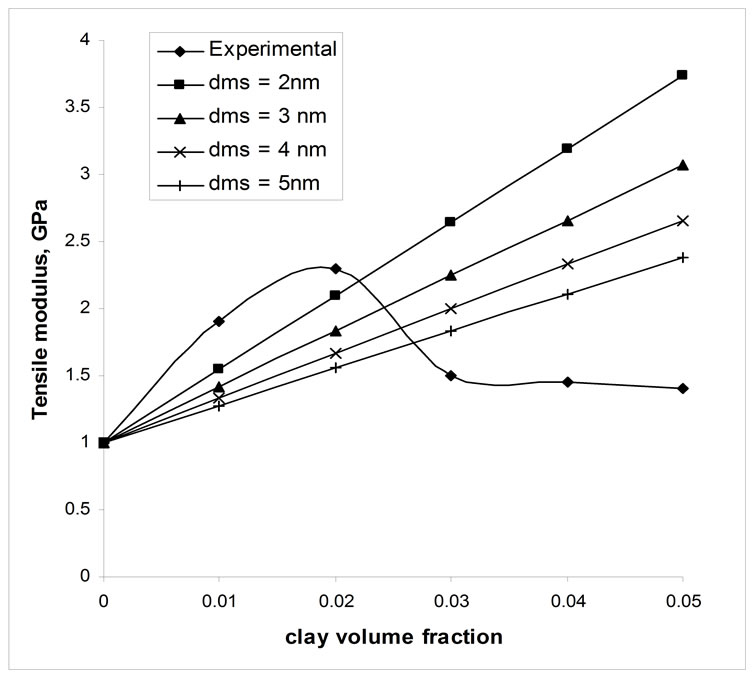
Figure 5. Comparison of tensile modulus of nanocomposites and stack model.
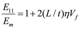
volume fraction; particle aspect ratio; and their orientation. In applications relevant to the present study, the particles and matrices are assumed to be linearly elastic, can be taken as isotropic or transversely isotropic. Here, Ep and Em denote the elastic modulus of the particle and the matrix respectively. Later, Tucker et al. [16] provides a good review of the application of several classes of micromechanical models to discontinuous fibre reinforced polymers. It is noted that, of the existing models, the widely used Halpin-Tsai equations give reasonable estimates for effective stiffness, but the Mori-Tanaka type models give the best results for large aspect-ratio fillers. The present study is focused on the prediction of longitudinal stiffness, E11; for composites filled with unidirectional disk-like particles. The Mori-Tanaka model is given by Equation (5).
 (5)
(5)
 is the shape factor which can be taken from Halpin-Tsai shape factor (Equation (3)), t is the thickness of the clay nanolayer (1 nm) and L is the length of the clay nanoclayer (nm). Figure 6 shows the comparison of experimental values with theoretical results for different values of clay length. The thickness of nanolayer ‘t’ is taken as 1 nm.
The modulus values increases as the length of clay nanoparticle increases. The theoretical prediction of modulus up to low clay volume fraction is better, however, at higher clay concentrations, there exists large variations in the experimental values and Mori Tanaka result. This suggests that other parameters are influencing the experimental trend. The length of clay layers are not the function of clay concentrations since same species of clays are used. Hence it is understood that net aspect ratio (length/thickness) has affected the aspect ratio. Also, stacking of clay nanolayers is high at higher clay concentration (intercalated structure). All these factors could have reduced the modulus at higher clay content. Mori -Tanaka formulation considers only the size, shape, aspect ratio and volume fraction of fillers, however, it does not consider the effect of net aspect ratio of fillers (which is predominant at higher clay content). In Mori-Tanaka formulation, the bahaviour of interface characteristics is also not considered, which is taken care in Takanayagi’s phase model.
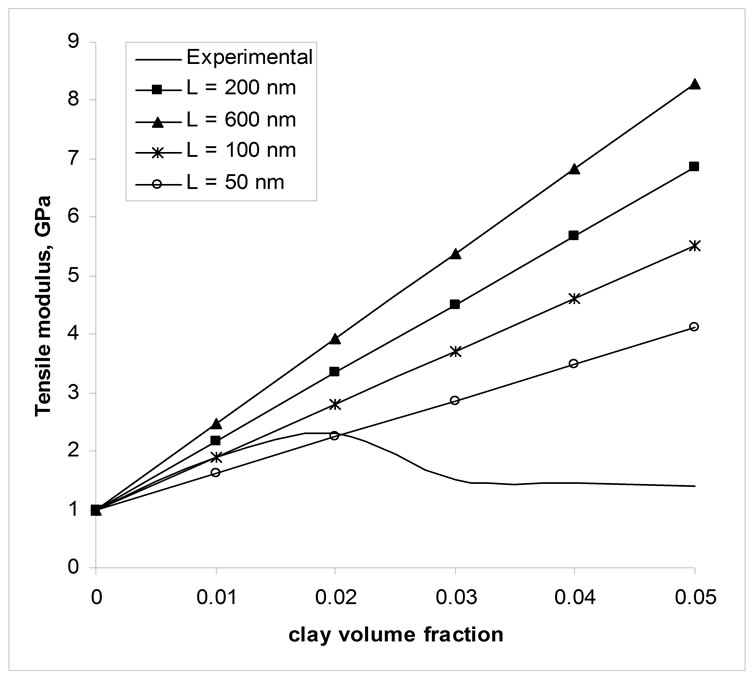
Figure 6. Comparison of modulus with Mori-Tanaka theory.
3.4. Takanayagi’s Two Phase and Interface Model
The phase model suggested by Takayanagi has widely been used to explain modulus of polymers, polymer blends and composites [16]. Two phase model describes the modulus of composites which consists of homogeneous rigid discontinuous phase and homogenous continuous matrix phase. When the dispersed particles approach a very small size, the specific surface area of the interfacial region is so large that it is comparable with or even larger than that of the dispersed phase. Recent work on polymer nanocomposites shows that the macromolecular chains intercalated in inorganic compounds are confined in a very small region and their behaviour is quite different from those in bulky polymers. It is found that these macromolecules are quite rigid. Based on this, an interface contribution of matrix and particle is taken in to account in Takayanagi’s model.
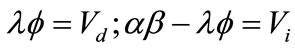
The moduli of the matrix, dispersed phase, and interface are Em, Ed and Ei respectively, and their corresponding volume fractions are Vm, Vd and Vi respectively. Figure 7 shows the distribution of particles in the matrix. The schematic of filler/matrix interface is also depicted. The system can be explained as a three-phase model in which the three phases are connected to each other in series and in parallel. The response of these three phases to a stress is schematically shown in Figure 8.
The three phase model as shown in Figure 8 is divided in to three regions which are connected in series as A, B and C. The elongation of these three regions under
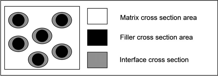
Figure 7. Schematic of cross-section view of polymer-parti- cle filled composites.
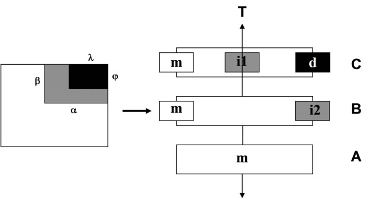
Figure 8. Equivalent model under tensile response.
the stress (T) loaded on the specimen are eA, eB and eC, respectively. In region A, only matrix with volume fraction VAm exists. In region B, the interface with volume fraction VBi and matrix with volume fraction VBm coexist in a parallel arrangement. In region C, the matrix with volume fraction VCm, the interface with volume fraction Vd coexists in a parallel arrangement. It is known that VAm + VBm + VCm = Vm, VBi + VCi = Vi.
The elongation in region A is
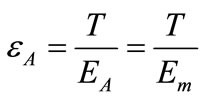 (6)
(6)
where EA is the modulus of the region A, i.e., Em.
The elongation in region B is:
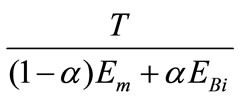 (8)
(8)
The elongation in region C is
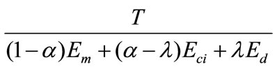 (9)
(9)
The total elongation in these three regions is
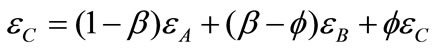
=  (10)
(10)
Where
 (11)
(11)
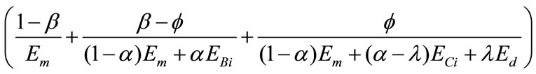
Since  /T = 1/Ec, where Ec is the modulus of the composites, Equation (10) becomes
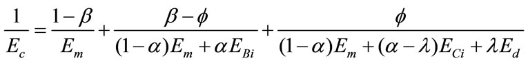 (12)
(12)
This equation can be understood by considering some special cases.
1) when  = Vd = 0, i.e. no dispersed phase and therefore no interfacial region, only a matrix exists, then Ec = Em
2) when  = 0, 1 – a = 0, i.e., b = 1, a = 1 and Vm = 0, i.e., the matrix phase does not exist. Here there is no interfacial region and dispersed phase giving Ec = Ed
3) when a – λ = b – j = 0, or a = – λ and b = j, Equation (12) reduces to
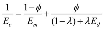 (13)
(13)
The Equation (13) describes the modulus of two-phase composites namely homogeneous rigid phase and homogeneous matrix phase. However, in nanoclay filled composites, the matrix particle interface has to be considered and this is given in 3-phase model.
3.4.1. Modulus of the Interfacial Region
The modulus of the interface in regions 1 and 2 are different from each other (shown in Figure 8). In the region 1, owing to the parallel arrangement of a number of volume units in the interfacial region, the modulus of this region could be expressed by:
 (14)
(14)
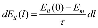
where Eil(l) is the modulus at region 1 with the distance l from the surface of the dispersed rigid phase. If a linear gradient distribution of the modulus along the normal direction of the surface is assumed, then
 (15)
(15)
After integration, the Equation (16) is obtained:
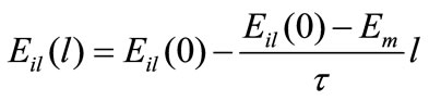 (16)
(16)
where Eil (0) is the modulus of the interface at the surface of the dispersed rigid phase and t is the thickness of the interface region. When l = 0, Eil (0) stands for the modulus of the interface, close to the surface of the fillers and it is a constant. Alternately, when l =t, Eil (t) represents the modulus at the edge of the interface next to the matrix, i.e., Em (Figure 9). If there exists linear decrease of Ef along l, then the modulus of the interface region l with thickness of t is then
 (17)
(17)
As seen in Figure 8, the region 2 (Block i2) connects with the dispersed phase at the top and connects with the matrix at the bottom. From top to bottom the modulus of these phase varies from Ei2(0) to Em. Block i2 can be treated as a series arrangement of a number of volume units and the modulus in this region varies with l.
It should be noted that EBi = Ei2, ECi = Eil. Eil or Ei2 could be another type of function depending on the interaction of the macromolecules with the surface of dis-
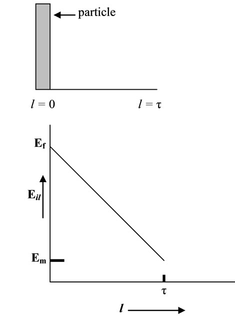
Figure 9. Variation of interface modulus along the normal of particle surface.
persed phase. In the present case it is assumed that modulus Eil and Ei2 are same.
3.4.2. Tensile Modulus of Polymer Nanocomposites
If the modulus in the interfacial region takes a linear gradient reduction along the normal direction of the surface of dispersed phase, Equation (13) would be
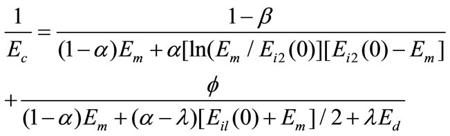
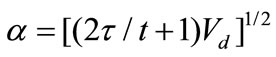
If a random orientation of the plate-like dispersed phase is considered with thickness = λ, length and width as ζ and ζ 1, the following conditions are assumed, i.e., a = b, j = λ. Each plate particle has two interface regions: Vd = λ and a2 – Vd = (2t/t)Vd, which can be arranged as
 (19)
(19)
The modulus of interfacial region is assumed to be
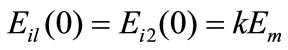 (20)
(20)
Where k represents the modulus ratio (1 < k < [Ed/Em]) of the neighboring interface surface of a dispersed particle. Thus the equation obtained is
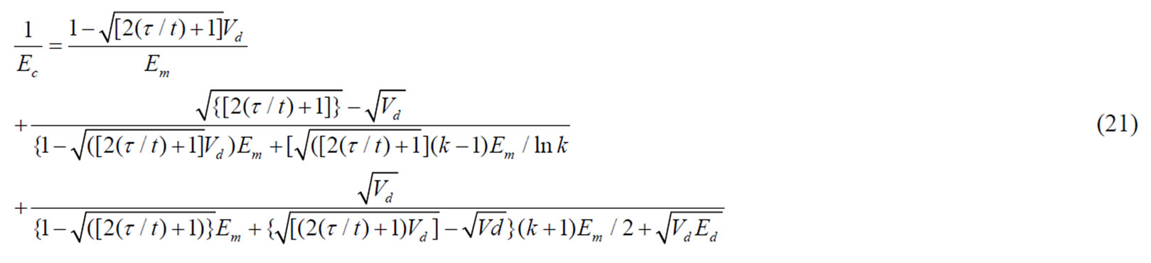
Using the above equation the effects of particle size, particle shape, thickness of interfacial region, modulus ratio of dispersoid phase to the matrix, and the k value on nanocomposites is studied.
3.4.3. Effect of k Value
k is the modulus ratio of the particle surface adjacent to the matrix and is usually in the range of 1 < k < (Ed/Em). Ec increases with the increase of k and the variation is shown in Figure 10. The result shows that for higher clay conent the experimental values better with theoretical values. Also the curve suggests that the interfacial modulus has considerable effect on tensile modulus of composite. At lower clay concentration, possibly interfacial moduli are higher or the model may not suit with experimental results.
3.4.4. Effect of Particle Size and Interface Thickness
The effect of particle size on the modulus of nanocomposites is studied and the results are shown in Figure 11. The thicknesses of layers are varied from 1 nm to 30 nm. Here the interface thickness is assumed as 10 nm and k as 30. By altering these parameters possibly some match between experimental and theoretical can be expected. Figure 12 shows the effect of interface thickness on composite modulus. This suggests interface thickness has some influence in nanocomposite modulus.
3.5. Optical Dispersion Parameters
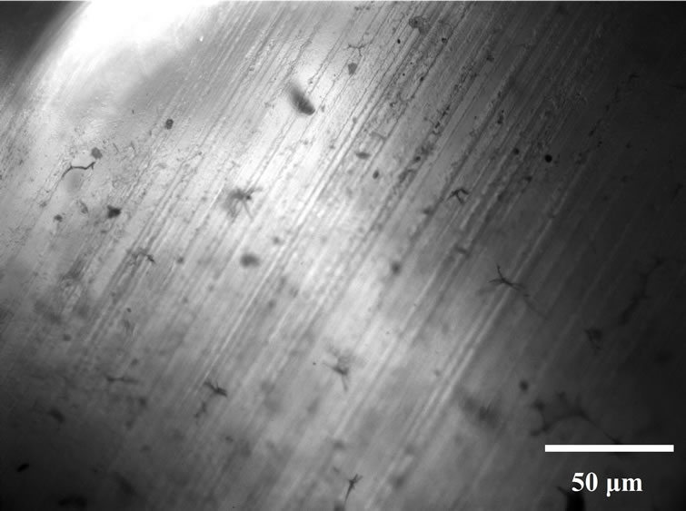
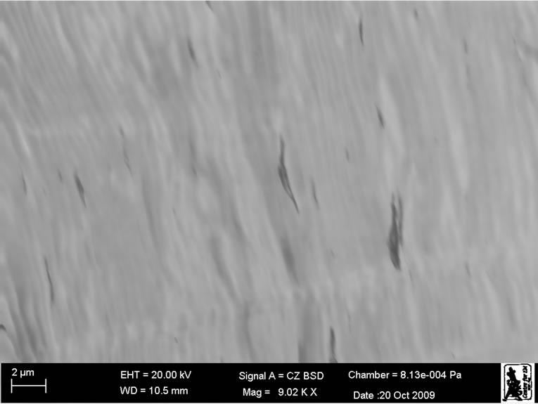
The above discussed theoretical models consider mostly the geometry and composition of composites. To some extent, they consider the interface characteristics in predicting the modulus values of composite series. Hence, most likely experimental and theoretical results do not match each other. In this section, optical dispersion parameters (namely: Agglomeration %, Exfoliation number, degree of dispersion) are taken in to consideration for predicting modulus values. These parameters are measured by viewing the composite material through Optical microscope (Figure 13) and Transmission Electron Microscope (Figure 14).
In Figure 13 of OM, the bright phase is the matrix phase and the dark phase is the particle phase. As the clay concentration increases the clay stacking becomes more and hence more aggregated clay phase is seen. Figure 14 shows the bright field TEM of PP-clay nanocomposites. Matirx phase represents the bright region and the dark phase represents the particle (clay) regions.
Agglomeration % (Agg. %) is the proportion of micron size agglomerates in Optical microscope, micron -size agglomerates larger than 5 microns are considered. The area lesser than 5 microns was analyzed using TEM images.
The Agg. % were calculated using OM and using the Equation (22)
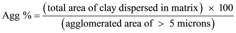 (22)
(22)
It is observed that Agg. % increases as clay concentration increases in polymer matrix. The exfoliation number (ξn) is calculated from TEM pictures (Figure 14) as per Equation (23).
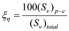 (23)
(23)
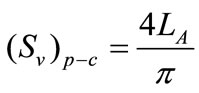
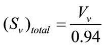
where (SV)P−C is the polymer-clay interfacial area per unit volume of the specimen and (SV)total is the total clay
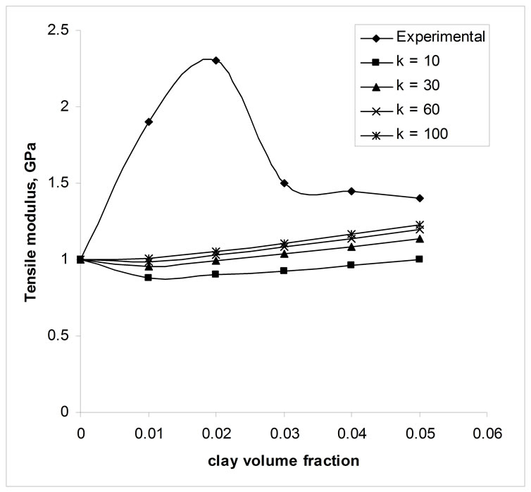
Figure 10. Effect of interface modulus.
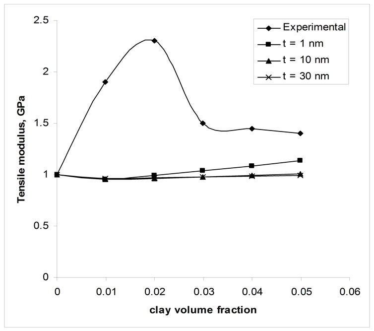
Figure 11. Effect of particle thickness.
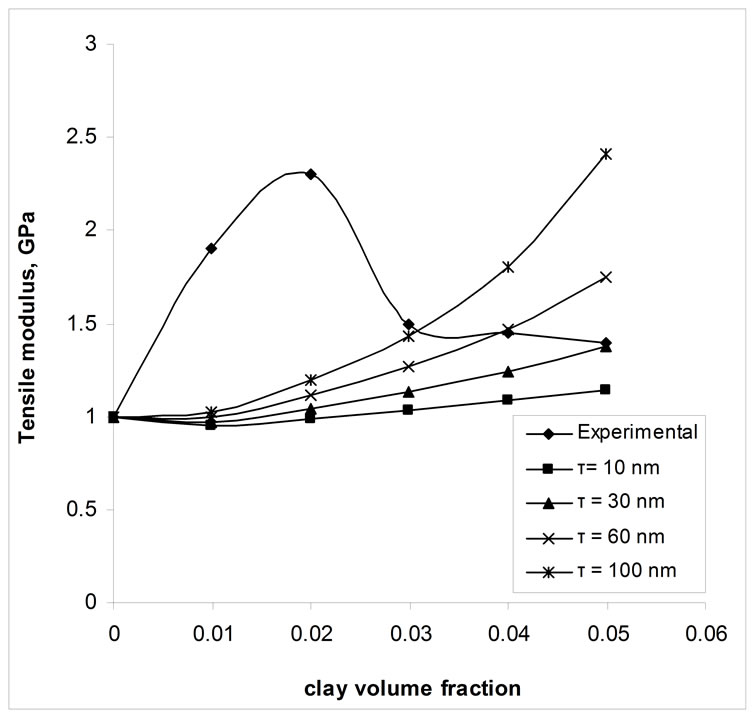
Figure 12. Effect of interface thickness.
 (a)
(a)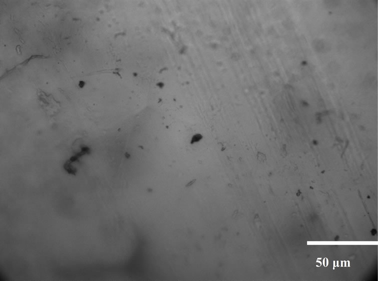 (b)
(b)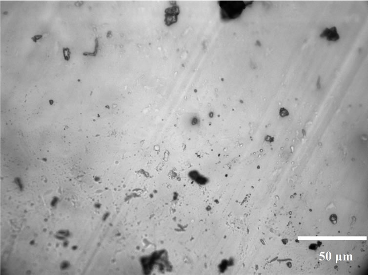 (c)
(c)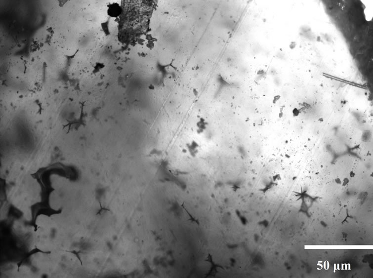 (d)
(d)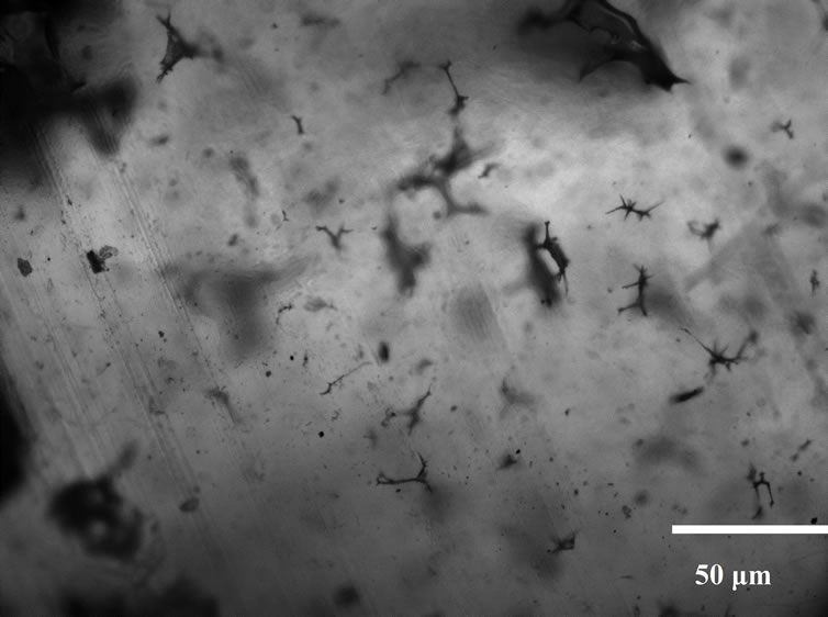 (e)
(e)
Figure 13. Optical microscope of PP with (a) 1%, (b) 2%, (c) 3%, (d) 4% and (d) 5% clay.
 (a)
(a)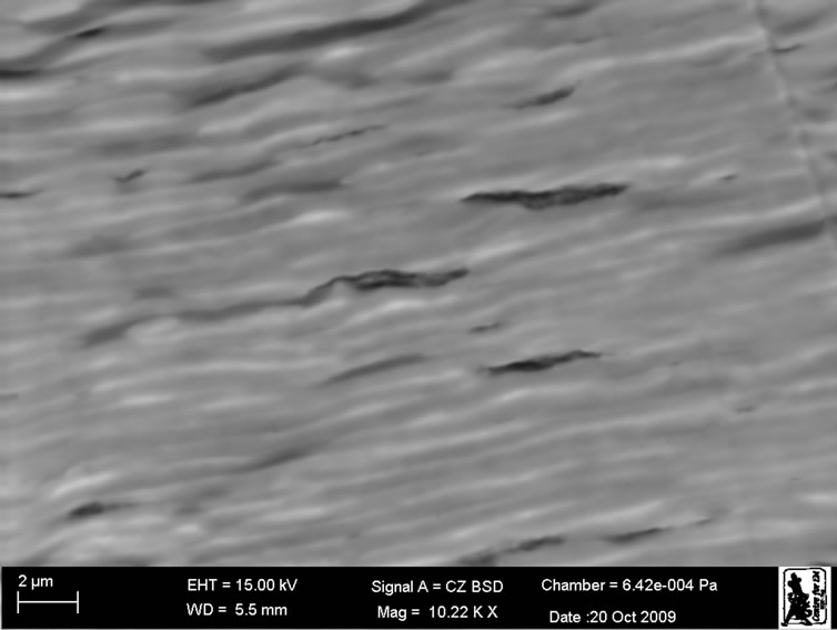 (b)
(b)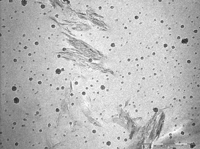 (c)
(c) (d)
(d) (e)
(e)
Figure 14. TEM of PP with (a) 1%, (b) 2%, (c) 3%, (d) 4% and (e) 5% clay.
 (24)
(24)
 (25)
(25)
where LA is the total length of perimeter of particles per unit area from TEM images, VV is the volume fraction of clay estimated from the area fraction of all particles from TEM images. The degree of dispersions (c) is calculated as per the Equation (26).
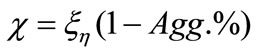 (26)
(26)
The values of these parameters are shown in Table 1. Figure 15 shows the experimental values and values obtained from dispersion parameters. These parameter were compared and it is observed that these parameters fit well with experimental results. The resulted disper-
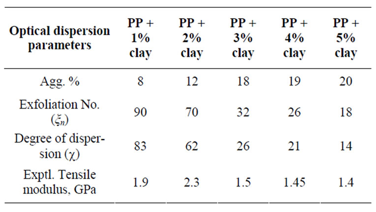
Table 1. Nanocomposite dispersion data and property.
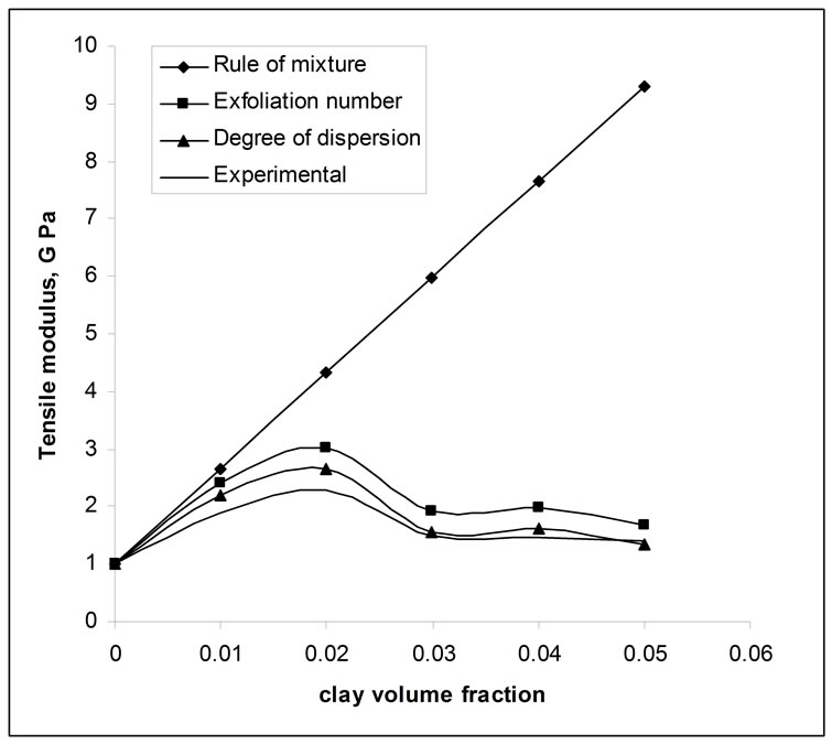
Figure 15. Comparison of rules of mixtures, experimental obtained values and analytical dispersion parameters.
sion parameter (Table 1) values are substituted with theoretical modulus from rules of mixtures and graphs are plotted. It is observed a close matching between dispersion parameters and experimental results.
4. Conclusions
The structural changes that are taking place in PP-nanoclay systems are quantified as optical dispersion parameters and were measured using TEM and OM image analysis. The dispersion parameters measured were exfoliation number (ξn), degree of dispersion (c) and agglomerate concentration (Agg. %). These parameters were substituted in rules of mixtures (parallel model) to predict tensile modulus of nanocomposites and observed a good correlation between experimental and theoretical tensile modulus. Further, the modulus prediction by these optical dispersions method is better than other standard models. This good correlation of optical dispersion parameters with experimental results shows positive goal towards successfully measurement of tensile modulus.
5. REFERENCES
- F. Perrin-Sarazin, M.-T. Ton-That, M. N. Bureau and J. Denault, “Microand Nano-Structure in Polypropylene /Clay Nanocomposites,” Polymer, Vol. 46, No. 25, 2005, pp. 11624-11634.
- B. Q. Chen and J. R.G. Evans, “Impact and Tensile Energies of Fracture in Polymer-Clay Nanocomposites,” Polymer, Vol. 49, No. 23, 2008, pp. 5113-5118.
- S. Pavlidou and C. D. Papaspyrides, “A Review on Polymer-Layered Silicate Nanocomposites,” Progress in Polymer Science, Vol. 33, No. 12, 2008, pp. 1119-1198.
- C. E. Powell and G. W. Beall, “Physical Properties of Polymer/Clay Nanocomposites,” Current Opinion in Solid State and Materials Science, Vol. 10, No. 2, 2006, pp. 73 -80.
- N. Sheng, M. C. Boyce, D. M. Parks, G. C. Rutledge, J. I. Abes and R. E. Cohen, “Multiscale Micromechanical Modeling of Polymer/Clay Nanocomposites and the Effective Clay Particle,” Polymer, Vol. 45, No. 2, 2004, pp. 487-506.
- G. Scocchi, P. Posocco, A. Danani, S. Pricl and M. O. Fermeglia, “To the Nanoscale, and beyond: Multiscale Molecular Modeling of Polymer-Clay Nanocomposites,” Fluid Phase Equilibria, Vol. 261, No. 1-2, 2007, pp. 366 -374.
- T. D. Fornes and D. R. Paul, “Modeling Properties of Nylon 6/Clay Nanocomposites Using Composite Theories,” Polymer, Vol. 44, No. 17, 2003, pp. 4993-5013.
- S. Boutaleb, F. Zaïri, A. Mesbah, M. Naït-Abdelaziz, J. M. Gloaguen, T. Boukharouba and J. M. Lefebvre, “Micromechanics-Based Modelling of Stiffness and Yield Stress for Silica/Polymer Nanocomposites,” International Journal of Solids and Structures, Vol. 46, No. 7-8, 2009, pp. 1716-1726.
- J.-J. Luo and I. M. Daniel, “Characterization and Modeling of Mechanical Behavior of Polymer/Clay Nanocomposites,” Composites Science and Technology, Vol. 63, No. 11, 2003, pp. 1607-1616.
- G. Tanaka and L. A. Goettler, “Predicting the Binding Energy for Nylon 6,6/Clay Nanocomposites by Molecular Modeling,” Polymer, Vol. 43, No. 2, 2002, pp. 541-553.
- Y.-P. Wu, Q.-X. Jia, D.-S. Yu and L.-Q. Zhang, “Modeling Young’s Modulus of Rubber-Clay Nanocomposites Using Composite Theories,” Polymer Testing, Vol. 23, No. 8, 2004, pp. 903-909.
- S. K. Basu and Tewari, “Transmission Electron Microscopy Based Direct Mathematical Quantifiers for Dispersion in Nanocomposites,” Applied Physics Letters, Vol. 91, No. 5, 2007, p. 053105.
- J. C. Halpin and J. L. Kardos, “The Halping-Tsai Equations: A Review,” Polymer Engineering and Science, Vol. 16, No. 5, 1976, pp. 344-352.
- D. A. Bruce and J. Bicerano, “Micromechanics of Nanocomposites: Comparison of Tensile and Compressive Elastic Modulii, and Prediction of Effects of Incomplete Exfoliation and Imperfect Alignment on Modulus,” Polymer, No. 43, No. 2, 2002, pp. 269-287.
- T. Mori and K. Tanaka, “Average Stress in Matrix and Average Elastic Energy of Materials with Misfitting Inclusions,” Acta Metallurgica, Vol. 21, No. 5, 1973, pp. 571-574.
- L. J. Xiang, K. J. Jiao, W. Jiang and B. Z. Jiang, “Tensile Modulus of Polymer Nanocomposites,” Polymer Engineering and Science, Vol. 42, No. 5, 2002, pp. 483-493.
Notation
α length fraction of interface
β width fraction of interface
λ length fraction of dispersoid
φ width fraction of dispersoid
χ degree of dispersions
ζ shape factor of filler
h modulus ratio factor
τ interface thickness
ξn exfoliation number
eA, eB, eC elongation in region A, B and C respectively
a length of clay platelet
k interface modulus (modulus ratio)
t nanoclay thickness
dms thickness of matrix in a stack
Ec Young’s modulus of composites
Em Young’s modulus of matrix
Ef Young’s modulus of filler
Es Stack modulus
Ep Youngs’s modulus of particle
Vf volume fraction of filler
Vm volume fraction of matrix
Ecl clay modulus in stack
Emi matrix modulus in stack
Vcl volume fraction of clay in stack
Vmi volume fraction of matrix in stack
L length of clay platelet
T applied load