Applied Mathematics
Vol.10 No.06(2019), Article ID:93194,17 pages
10.4236/am.2019.106033
Diffraction of Surface Harmonic Viscoelastic Waves on a Multilayer Cylinder with a Liquid
Safarov Ismoil Ibrohimovich1, Kulmuratov Nurillo Rakhimovich2, Teshayev Muhsin Khudoyberdiyevich3*, Kuldashov Nasriddin Urinovich1
1Tashkent Institute of Chemistry and Technology, Tashkent, Republic of Uzbekistan
2Navoi State Mining and Metallurgical Institute, Navoi, Republic of Uzbekistan
3Bukhara Engineering-Technological Institute, Bukhara, Republic of Uzbekistan

Copyright © 2019 by author(s) and Scientific Research Publishing Inc.
This work is licensed under the Creative Commons Attribution International License (CC BY 4.0).
http://creativecommons.org/licenses/by/4.0/


Received: April 1, 2019; Accepted: June 21, 2019; Published: June 24, 2019
ABSTRACT
An infinitely long circular cylinder, consisting generally of a finite number of coaxial viscoelastic layers, surrounded by a deformable medium is considered. The dynamic stress—the deformed state of a piecewise-homogeneous cylindrical layer from a harmonic wave is investigated. The numerical results of stress, depending on the wavelength are obtained.
Keywords:
Viscoelasticity, Fluid, Frequency, Longitudinal and Transverse Wave, Shell, Plane Strain

1. Introduction
During seismic impacts, modern underground pipelines operate under conditions of not only static but also dynamic loads, which are accompanied by large damage and even failure of the whole system [1] - [6] . In the case of a sufficiently long cavity, the impact perpendicular to its longitudinal axis, the environment surrounding the cavity and the lining are in conditions of plane deformation, and the task of determining the stress state of the array and lining reduces to a flat problem of the dynamic theory of elasticity (and whether visco-elasticity) [7] [8] [9] [10] . In [11] , the problem of stress concentration in an infinite linearly elastic cavity near a circular cavity with the propagation of longitudinal harmonic waves was solved. The solution of the diffraction problem for a harmonic transverse wave was obtained in [12] . This paper investigates the interaction of cylindrical stress waves with a cylinder, which in the general case consists of a finite number of coaxial viscoelastic layers. Due to the fact that long-term seismic waves, as a rule, exceed the characteristic dimensions of the cross section designs (for example, diameter D), therefore, when solving diffraction problems,
it is necessary to consider long-wave effects ( , is the wavelength). With longer wavelengths ( ) maximum coefficients of dynamic concentrations turned out to be 5% - 10% more than with the corresponding biaxial static loaded ( ) [13] . At dynamic stress concentrations are significantly lower than static. In [14] , it was shown that the difference in
dynamic stress concentrations in the case of a rigid inclusion and cavity can be attributed to the possibility of propagation of generalized Rayleigh-type waves on a concave free cylindrical surface of the cavity. A significant contribution to the calculation of flexible pipelines was made in [15] [16] , which investigated such important issues as accounting without a backing zone and determining the stability of underground pipelines. There are a large number of authors who have applications in other branches of technology who can be successfully applied to the calculation of underground pipelines. These works are devoted to the study of the stress distribution in plastic, weakened by a reinforced bore, operating under plane strain conditions. The most significant research in this area can be attributed to the work that solved the problem in stretching a plate in which a ring is embedded or soldered.
2. Problem Statement and Basic Relations
In this paper, the interaction of a cylindrical stress wave by parallel-layered elastic layers with a liquid is investigated. It is assumed that the linear source in Figure 1 is a continuous source of dilatation (or transverse) stress waves with an angular velocity ω and amplitude (or ), and the layered package is a thick-walled and thin-walled layers of the cylinder. In describing the movement of thin-walled elements, the equations of the theory of such shells are used, which are based on the Kirchhoff-Love hypotheses. For thin-walled layers, the original equations are the linear theory of elasticity. The numbering of the layers is the product in ascending order of their radii from k = 1 to k = N (Figure 1). The value characterizing the properties and the state of the elements correspond to the values , where K is the elastic layer enclosed between K-1 and K-m layers. The environmental parameters are denoted by the indices K = N (Figure 1). Under the assumption of a generalized plane-deformed state, the equation of motion in displacements has the form [1]
(1)
where and ( , —relate to the environment, —to layer) operator moduli of elasticity [13]

Figure 1. The design scheme of layered cylindrical bodies in a deformable medium.
—Volume force density vector ( ); —some function; —density of materials, and —relaxation core, —instantaneous elastic moduli of viscoelastic material, —displacement vector which depends on . At pressures up to 100 MPa, the movement of the fluid in is satisfactorily described by the wave velocity of the particle particles [14]
. (2)
where ; Со—acoustic velocity of sound in a fluid. Potential and the fluid velocity vector are dependent . Fluid pressure is determined using the linearized Cauchy-Lagrange integral —fluid pressure on the wall of the cylindrical layer and ρо-fluid density Under the condition of continuous flow of fluid, the normal component of the velocity of the fluid and the layer on the surface of their contact r = R0 must be equal
. (3)
where —moving the layer along the normal. On the contact of two bodies r = Rj equal displacements and stresses (fixed contact condition)
(4)
Note that in the case of sliding ground contact over the pipe surface, the last Equation in (4) takes the form [16] :
.
where and —radial and tangential stresses in the j-th viscoelastic body; and —radial and tangential displacement of the j-th body. The solution of the wave Equation (1) in the displacement potentials satisfies at infinity the Summerfield radiation condition [14] :
, (5)
.
As , natural oscillations by the first and third conditions (5) are not fulfilled, therefore, the shortened Sommerfeld conditions at infinity are set, which in detail in [14] was considered.
If in place the equation of motion (1) is used cylindrical shells, then the equation of motion of shells in a flat formulation is:
(6)
where u and W- longitudinal and transverse displacements respectively:
Shell radius , —shell density, —shells Puasson ratio, —shell thickness, —shell elastic modulus, and —normal and tangent components of the reaction from the environment.
The contact between the shell and the environment can be hard or sliding:
(7)
Consider a longitudinal wave generated by a longitudinal source of expansion waves located at (Figure 1). The displacement potentials of the incident expansion wave can be represented as [15]
. (8)
where —is the divergent functions of Henkel (the first kind of zero order); —expansion wave amplitude; —compression wave number; , , w—circular frequency. In the absence of an incident wave (6), the natural oscillations of a reinforced bore located in a viscoelastic medium are considered.
3. Solution Methods
The problem is solved in displacement potentials, for this we present the displacement vector in the form:
where —longitudinal wave potential; —vector potential of transverse waves.
The basic equations of the theory of visco elasticity (1) for this problem of plane strain are reduced to the following equation
(9)
where —differential operators in cylindrical coordinates and — Poisson’s ratio.
At infinity, potentials of longitudinal and transverse waves with satisfy the Summerfield radiation condition (5).
The solution of Equation (9) can be sought in the form:
(10)
where and —complex function which is solving the following Equations (10)
(11)
where , ,
, ,
, .
The solution of Equation (9) with regard to (11) is expressed in terms of Henkel functions of the 1st and 2-nd kind of the nth order:
(12)
where and —decomposition coefficients, which are determined by the corresponding boundary conditions; and —respectively, the Henkel function of the 1st and 2nd kind of the nth order .
Solution (12) with satisfies at infinity the Somerfield radiation condition (5) and is represented as:
Solving problem (2) with satisfies the condition of limiting the force factors [10] and it follows that
The full potential can be determined by imposing the potentials of the incident and reflected waves. Thus, the displacement potentials will be
(13)
To determine the stress-strain state, it is first necessary to express the incident wave through wave functions (13). Using the geometric construction in Figure 1 and moving from the coordinates to coordinates in the area of
.
where , —cylindrical Bessel function of the first kind.
It follows that voltages and offsets can easily be expressed in terms of displacement potentials [15]
(14)
Displacement and stresses for the case of a compression wave falling on a layer it turns out.
Substituting (13) into (14) after considering (11), we obtain the following expression for displacement and stress:
(15)
where
where .
The construction of a formal solution does not meet fundamental difficulties, but the study of such a solution requires a huge amount of computation. The tasks are reduced to solving inhomogeneous algebraic equations with complex coefficients
. (16)
where {q} is a vector column containing arbitrary constants; {F}—vector column of external loads; [C] is a square matrix, the elements of which are expressed through the functions of Bessel and Henkel. Equation (13) is solved by the Gauss method with the selection of the main element. In the work of movement and stress is reduced in dimensionless types
In the case when , and , we get holes (r = R0) that are in infinitely elastic medium ( , ). The boundary (r = R0) is stress free, i.e. no liquid. In this case, the circumferential voltage on the surface of the cavity is reduced to the following:
(17)
where
Now consider some limiting cases.
With :
And : , the asymptotic formulas of Hankel of the 1st and 2nd kind were used [17] . If in expression (17) Z tends to infinity, then we can use the asymptotic expansions of the Henkel function for large values of the argument [17] (α- is a finite)
(18)
This expression completely coincides with the expressions obtained by [17] for a plane incident wave. If the wave number tends to zero, then the limiting process describes static solutions for long waves. This limiting process allows us to use approximating expressions for the Henkel functions for small values of the argument (Z is finite)
(19)
This solution exactly coincides with the solution of the static problem obtained in [18] . If the cylindrical cavity contains an ideal fluid, then the ring stresses take the form
where . At , then it turns out the solution of a static problem
In the limiting processes in expressions (15) and (16) is described by physical results, is given in Table 1. The stress concentration coefficient is determined by the following formulas
. (20)
where .
If we take the fluid into account, then using (2), (3) and (15) we can determine the corresponding stresses and . In the absence of an incident wave (6), the natural oscillations of an unsupported (or reinforced) hole located in the medium are considered.
At the boundary r = R, we set a voltage-free condition, i.e.
. (21)
Substituting (12) into (21), we obtain the frequency equation
. (22)
where

Table 1. Information on limiting processes.
Frequency Equation (22) is solved numerically, i.e. Muller method. The complex eigenfrequencies are given in Table 2. In the table of the first column correspond the complex frequency , second , third and fourth, columns .
The partial equation, for differential Equations (6), under the condition of a sliding contact, takes the form:
(23)
where
—Rod wave velocity
(24)
In this case, we obtain asymmetric vibrations of the cylindrical shell, which are described by the expression
. (25)
where (the index “0” corresponds to the shell, and “1” to the environment). If we use the asymptotic expression of the Henkel function with , then for the zero and first order we obtain the expression of the complex natural frequencies
Table 2. The dependence of the complex natural frequencies of the cylindrical hole.
(26)
To obtain complex and imaginary natural frequencies, the following condition must be met
(27)
To fulfill the first condition, the modulus of elasticity E must satisfy the inequality
(28)
A similar condition is set for η:
The numerical values of asymmetric (n = 0) natural frequencies are given in Table 3 for different values of E(Е1/E0).
4. Numeric Results
For given incident wave, voltage and displacement are determined by the rows described by expressions (12) - (17) in the case of hard contact. The calculations were performed on the Mat lab computer program complex; the series were calculated with an accuracy of 10−8. All expressions for stresses and displacements are:
. (29)
As can be seen, the solution of the problem is expressed through the special functions of the Bessel and Henkel of the 1st and 2nd kind. With the increase in their argument, the series (12) - (17) converges. Therefore, on the basis of numerical experiments, it has been established that the accuracy of 5 - 6 members
of the series has reached 10−6 - 10−8. As the relaxation core of a viscoelastic material, let’s take a three-parameter core Rizhanitsen-Koltunova
[19] , which has a weak singularity, where —parameters materials [19] .
Table 3. The dependence of the complex natural frequencies of ax symmetric vibrations of cylindrical shells on E.
Take the following parameters: . To study the stress concentration on the free surface, we use the absolute values of the complex value and relations (18) and (19). The magnitude of the complex function depends on the wave number α, angle θ distances , Poisson’s ratio, Young’s module, densities, geometrical parameters R and Z. If all the characteristics (Figure 1) of the mechanical system are the same ( ; ; ), then the problem of the interaction of cylindrical waves with cylindrical cavities is considered. Figure 2 shows the plot of the stress concentration factor depending on θ at
.
Figure 2 shows that the influence of the proximity of the source lies in moving the maximum value to the point where the line drawn from the source touches the boundary of the cavity.
For the stress concentration coefficients, we will use the absolute value of the complex value (21). Figure 3 shows the change depending on the wave number at different values , which quickly aim for a solution for a plane wave when . This means that when the source is at a
distance of five radii from the cavity, the high frequency nature of the change can be approximated by a solution for a plane wave. Further, all values approach the same asymptote. The largest difference between the solution for a plane wave ( ) and the solution under consideration is in the . Легко видеть, что когда , dynamic solution for the case of a plane wave is reduced to a static value ( ), i.e. .
A similar but more pronounced change is noted for at ( ) (Figure 4). When , solution for dynamic source with values
again reduced to a solution for a plane wave. When Z/R = 2 (Figure 3) the dynamic concentration curve differs from static to 15%. When Static and dynamic stress state results are radically different at close source distances (Z/R = 2). With R/Z > 50 the impact of the cylindrical source unfolds as a plane wave, i.e. you can ignore the radius of curvature of the wave. Similar results were obtained for a cylindrical cavity with an ideal fluid [20] . The results of the calculations are shown in Figure 5. It can be seen from the figure that the voltage
values strongly depend on the parameter . And also there is a resonant
phenomenon. Calculation results ( ) natural oscillations are shown in Table 2. As the table shows, with the increase in the number of waves around the circumference, the corresponding complex frequencies increase.
The complex frequencies consist of two parts, the real ( ) and imaginary parts ( ) which means natural frequencies and damping factors. Frequency equations (23) depends only on the parameter (Poisson’s ratio). With increasing Poisson’s ratio within real and imaginary parts of the complex frequency changes to 27%. With the environment becomes incompressible, the attenuation is naturally absent. The existence of an imaginary value of the natural frequency means that the oscillatory processes in the system are only damped. The imaginary natural frequencies turn out to depend on the longitudinal and transverse speeds, as well as the whole radius.
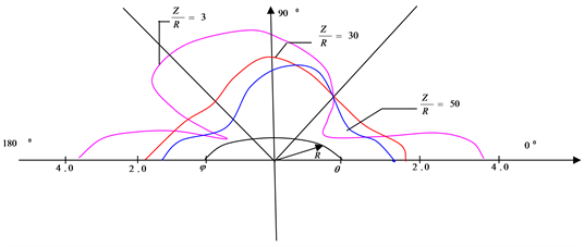
Figure 2. Effect of source proximity on voltages depending on the at different values of

Figure 3. depending on the (wave number) when Math_245#

Figure 4. Value depending on the ( ).

Figure 5. Dependency from (wave number).
The existence of a discrete frequency plays an important role for the calculation of underground pipelines located in the ground environment.
The obtained numerical results are presented in the form of tables and figures. The appearance of an additional free surface mainly thickens and reduces the Eigenvalue frequency by 10% - 16%. The existence of a natural frequency means that Rayleigh waves can occur in the vicinity of the free surface of a cylindrical hole. Thus, according to (28) with the real part of the complex frequency does not exist.
As we see, the real parts of the natural frequency vanish, and the behavior of the imaginary parts remains unchanged. The obtained numerical results are confirmed by the condition (25).
5. Conclusions
1) The task of diffraction of harmonic waves in a cylindrical body is solved in displacement potentials. Displacement potentials are determined from solutions of the Helmholtz equation. Arbitrary constants are determined from the boundary conditions that are put between the bodies. As a result, the task is reduced to a system of inhomogeneous algebraic equations with complex coefficients, which are solved by the Gauss method with the selection of the main element.
2) Contour stresses σθθ on the free surface of cylindrical bodies reach their maximum value in —when exposed to longitudinal waves, and —shear waves. Contour stresses σθθ when subjected to transverse harmonic waves, are 15% - 20% more than those when subjected to longitudinal waves.
3) When the source of harmonic waves is at a distance of five radii ( ) from a cylindrical body, the high-frequency nature of changes in loop stresses σθθ (on the inner free surface), is well approximated by the solution for a flat ( ) waves. Further, all values approach the same asymptote.
4) Numerical results show that the dynamic stress concentration factors near cylindrical bodies depend on the distance between the source and the body, the wave number for the cylinder and the medium; physico-mechanical parameters of the environment and the body.
5) Consideration of the viscous properties of the material of the environment when calculating the effect of seismic waves reduces stress and displacement by 10% - 15%. Calculations show that for fixed values of the amplitudes and the duration of the incident wave with increasing acoustic parameters of the fluid, the deflections and efforts also moderately increase. In the region of the long waves, the stress distribution of a pipe with and without liquid differs by up to 15%, and in the region of short waves, in some values of frequency, they differ by up to 40%. With a hole with a lining, the stress in the soil will be less than for the case of a hole without reinforcement. On the other hand, the amplification will be subjected to stresses from seismic loads and must withstand them.
6) The statement of the problem is proposed: natural oscillations of cylindrical bodies being in a deformable medium. The task is to find those ( —real and —imaginary parts of complex eigenfrequencies), in which the system of equations of motion and shortened radiation conditions have a nonzero solution in the class of infinitely differentiable functions. It is shown that the task has a discrete spectrum.
Conflicts of Interest
The authors declare no conflicts of interest regarding the publication of this paper.
Cite this paper
Ibrohimovich, S., Rakhimovich, K.N., Khudoyberdiyevich, T.M. and Urinovich, K.N. (2019) Diffraction of Surface Harmonic Viscoelastic Waves on a Multilayer Cylinder with a Liquid. Applied Mathematics, 10, 468-484. https://doi.org/10.4236/am.2019.106033
References
- 1. Guz, A.N., Kubenko, V.D. and Cherevko, M.A. (1978) Diffraction of Elastic Waves. Science Dumka, Kiev, 307 p.
- 2. Safarov, I.I. and Umarov, A.O. (2014) The Impact of Longitudinal and Transverse Waves on Cylindrical Layers with a Liquid. Perm University Bulletin. Mathematics. Mechanics. Informatics, 3, 69-75.
- 3. Safarov, I.I., Akhmedov, M.Sh. and Umarov, A.O. (2014) Dynamic Stresses and Mixing near a Cylindrical Reinforced Cavity from a Plane Harmonic Wave. Journal “Prospero” (Novosibirsk), 3, 57-61.
- 4. Safarov, I.I., Teshaev, M.Kh. and Boltaev, Z.I. (2017) Distribution of Harmonic Waves in Expansion Plastic and Cylindrical Viscoelastic Bodies. Open Science Publishing, Raleigh, 218 p.
- 5. Strelchuk, N.A., Slavin, O.K. and Shaposhnikov, V.N. (1971) Investigation of the Dynamic Stress State of Tunnel Lining under the Influence of Blast Waves. Building and Architecture, Moscow, No. 9, 129-136.
- 6. Rashidov, T.R., Hozhimatov, G.Kh. and Mardonov, B.M. (1975) Oscillations of Structures Interacting with the Ground. Fan, Tashkent, 174 p.
- 7. Rashidov, T.R., Sagdiev, H. and Safarov, I.I. (1989) On Two Main Methods for Studying the Seismic Stress State of Underground Structures under the Action of Seismic Waves. Reports of the Academy of Sciences, Tashkent, 6, 13-17.
- 8. Muborakov, Ya.N. (1987) Seismic Dynamics of Underground Structures of the Shell Type. Fan, Tashkent, 192 p.
- 9. Rashidov, T.R. (1973) Dynamic Theory of Seismic Resistance of Complex Systems of Underground Structures. Fan, Tashkent, 182 p.
- 10. Rashidov, T.R., Dorman, I.Ya. and Ishanhodzhaev, A.A. (1975) The Seismic Resistance of Tunnel Structures of the Metro. Transport, M., 120 p.
- 11. Muborakov, Ya.N. and Safarov, I.I. (1990) On the Basic Methods of Studying the Stress-Strain State of Underground Cylindrical Structures When Interacting with Elastic Waves. Collection: Durability of Engineering Structures under Seismic and Pulse Effects. Fan, Tashkent.
- 12. Muborakov, Ya.N. and Safarov, I.I. (1988) Assessment of the Seismic State of Underground Structures by the Method of Wave Dynamics. In: Seismodynamics of Buildings and Structures, Fan, Tashkent, 114-122.
- 13. Koltunov, M.A. (1976) Creep and Relaxation. Higher School, M., 277 p.
- 14. Safarov, I.I. (1992) Collisions and Waves in Dissipatively Non-Fertile Environments and Constructions. Fan, Toshkent, 250 p.
- 15. Mun, P. (1962) The Influence of the Curvature of Spherical Waves on the Concentration of Dynamic Stresses. Applied Mechanics, 2, 93.
- 16. Mente, M. (1963) Dynamic Stresses and Displacement in the Vicinity of a Cylindrical Discontinuity Surface from a Plane Harmonic Shear Wave. Applied Mechanics, 30, 117-126.
- 17. Ilyushin, A.A., Rashidov, T.R., et al. (1985) The Effect of Seismic Waves on Underground Pipelines. Proceedings of the International Scientific Conference: Friction, Wear and Lubricants, Tashkent, 22-26 May 1985, 128-132.
- 18. Gorshkov, A.G. (1981) Non-Stationary Interaction of Plates and Shells with Continuous Media. RHDL Proceedings of the Academy of Sciences. Fur. Solids, No. 4, 177-189.
- 19. Avliyakulov, N.N. and Safarov, I.I. (2007) Modern Problems of Statics and Dynamics of Underground Pipelines. Fan, Tashkent, 306 p.
- 20. Bozorov, M.B., Safarov, I. and Shokin, Yu.I. (1996) Numerical Simulation of Oscillations of Dissipatively Homogeneous and Inhomogeneous Mechanical Systems. Novosibirsk, 189 p.