Applied Mathematics
Vol.07 No.15(2016), Article ID:70630,17 pages
10.4236/am.2016.715147
Rothe’s Fixed Point Theorem and the Controllability of the Benjamin-Bona-Mahony Equation with Impulses and Delay
Hugo Leiva1, Jose L. Sanchez2
1Department of Mathematics, Louisiana State University, Baton Rouge, USA
2Departamento de Matemática, Universidad de Los Andes, Caracas, Venezuela

Copyright © 2016 by authors and Scientific Research Publishing Inc.
This work is licensed under the Creative Commons Attribution International License (CC BY 4.0).
http://creativecommons.org/licenses/by/4.0/


Received: May 7, 2016; Accepted: September 13, 2016; Published: September 16, 2016
ABSTRACT
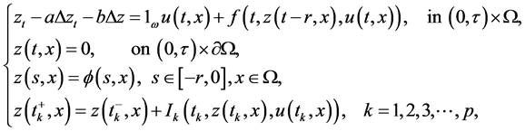
For many control systems in real life, impulses and delays are intrinsic phenomena that do not modify their controllability. So we conjecture that under certain conditions the abrupt changes and delays as perturbations of a system do not destroy its controllability. There are many practical examples of impulsive control systems with delays, such as a chemical reactor system, a financial system with two state variables, the amount of money in a market and the savings rate of a central bank, and the growth of a population diffusing throughout its habitat modeled by a reaction-diffusion equation. In this paper we apply the Rothe’s Fixed Point Theorem to prove the interior approximate controllability of the following Benjamin-Bona-Mahony (BBM) type equation with impulses and delay
 where
where  and
and  are constants,
  is a domain in
 ,
,  is an open non- empty subset of
 ,
,  denotes the characteristic function of the set
 , the distributed control
 ,
,  are continuous functions and the nonlinear functions
  are smooth enough functions satisfying some additional conditions.
Keywords:
Interior Approximate Controllability, Benjamin-Bona-Mahony Equation with Impulses and Delay, Strongly Continuous Semigroup, Rothe’s Fixed Point Theorem

1. Introduction
For many control systems in real life, impulses and delays are intrinsic phenomena that do not modify their controllability. So we conjecture that under certain conditions the abrupt changes and delays as perturbations of a system do not destroy its controllability. There are many practical examples of impulsive control systems with delays, such as a chemical reactor system, a financial system with two state variables, the amount of money in a market and the savings rate of a central bank, and the growth of a population diffusing throughout its habitat modeled by a reaction-diffusion equation. One may easily visualize situations in these examples where abrupt changes such as harvesting, disasters and instantaneous stocking may occur. These problems can be modeled by impulsive differential equations with delays, and one can find information about impulsive differential equations in Lakshmikantham [1] and Samoilenko and Perestyuk [2] .
The controllability of impulsive evolution equations has been studied recently by several authors, but most of them study the exact controllability only. For example, D. N. Chalishajar [3] studied the exact controllability of impulsive partial neutral functional differential equations with infinite delay and S. Selvi and M. Mallika Arjunan [4] studied the exact controllability for impulsive differential systems with finite delay. For approximate controllability of impulsive semilinear evolution equation, Lizhen Chen and Gang Li [5] studied the approximate controllability of impulsive differential equations with nonlocal conditions, using measure of noncompactness and Monch Fixed Point Theorem, and assuming that the nonlinear term  does not depend on the control variable. Recently, in [6] - [10] , the approximate controllability of semilinear evolution equations with impulses has been studied by applying Rothe’s Fixed Point Theorem, showing that the influence of impulses do not destroy the controllability of some known systems like the heat equation, the wave equation, the strongly damped wave equation. More recently, in [11] the approximate controllability of the heat equation with impulses and delay has been studied.
The approximate controllability of the linear part of the Benjamin-Bona-Mahony (BBM) equation was proved in [12] . This result was used to study the controllability of the nonlinear BBM equations in [13] , which could serve as a basis for studying the BBM equation under the influence of impulses and delays
 (1)
(1)
where  and
and  are constants,
  is a domain in
 ,
,  is an open non- empty subset of
 ,
,  denotes the characteristic function of the set
 , the distributed control
 ,
,  are continuous functions. Here
  is the delay and the nonlinear functions
  are smooth enough and satisfy
 (2)
(2)
 (3)
(3)
 ,
,  ,
,
and

One natural space to work evolution equations with delay and impulses is the Banach space

where  and
and , endowed with the norm

with

We shall denote by C the space of continuous functions:

endowed with the norm

Definition 1.1. (Approximate Controllability) The system (1) is said to be approximately controllable on  if for every
  and
and ,
,  there exists
  such that the mild solution
  of (1) corresponding to u verifies:

where

As a consequence of this result we obtain the interior approximate controllability of the semilinear heat equation by putting  and
and .
.
We also study the approximate controllability of the corresponding linear system
 (4)
(4)
by applying the classical Unique Continuation Principle for Elliptic Equations (see [14] ) and the following lemma.
Lemma 1.1. (see Lemma 3.14 from [15] , p. 62) Let  and
and  be sequences of real numbers such that:
 . Then

if and only if

The approximate controllability of the system (1) follows from the approximate controllability of (4), the compactness of the semigroup generated by the associated linear operator, the conditions (2) and (3) satisfied by the nonlinear term  and the following results:
Proposition 1.1. Let  be a measure space with
  and
and . Then
  and
and
 (5)
(5)
Theorem 1.1. (Rothe’s Fixed Theorem, [16] - [18] ) Let E be a Banach space and  be a closed convex subset such that the zero of E is contained in the interior of B. Consider
  be a continuous mapping with
a)  is compact.
b)  (
( , where
  denotes the boundary of B.
Then there is a point  such that

2. Abstract Formulation of the Problem
In this section we choose a Hilbert space where system (1) can be written as an abstract differential equation with impulses and delay; to this end, we consider the following notations:
Let  and consider the linear unbounded operator
  defined by
 , where

The operator A has the following very well known properties (see N. I. Akhiezer and I. M. Glazman [19] ): the spectrum of A consists of eigenvalues
 (6)
(6)
each one with finite multiplicity  equal to the dimension of the corresponding eigenspace. Therefore:
a) There exists a complete orthonormal set  of eigenvectors of A.
b) For all  we have
 (7)
(7)
where  is the inner product in Z and
 (8)
(8)
So,  is a family of complete orthogonal projections in Z and
 (9)
(9)
c)  generates the analytic semigroup
  given by
 (10)
(10)
Consequently, the system (1) can be written as abstract differential equations with impulses and delay in Z:
 (11)
(11)
where ,
,  ,
,  ,
,  is a bounded linear operator,
  is defined by
  and the functions
 ,
,  are defined by

 .
.
On the other hand, from conditions (2) and (3) we get the following estimates.
Proposition 2.1. Under the conditions (2)-(3) the functions ,
,  , defined above satisfy
  and
and :
:
 (12)
(12)
 (13)
(13)
Since  and
and  (
( is the resolvent set of A), then the operator:
 (14)
(14)
is invertible with bounded inverse
 (15)
(15)
Therefore, the systems (11) and its linear part can be written as follows, for 
 (16)
(16)
 (17)
(17)
Moreover,  and
and  can be written in terms of the eigenvalues of A:
 (18)
(18)
 (19)
(19)
Therefore, if we put  and
and , systems (16) and (17) can be written in the form:
 (20)
(20)
 (21)
(21)
and the functions F defined above satisfy:
 . (22)
Now, we formulate two simple propositions.
Proposition 2.2. ( [12] ) The operators  and
and  are given by the following expressions
 (23)
(23)
 (24)
(24)
Moreover, the following estimate holds
 (25)
(25)
where
 (26)
(26)
Observe that, due to the above notation, systems (20)-(21) can be written as follows
 (27)
(27)
 (28)
(28)
where .
.
3. Preliminaries on Controllability of the Linear Equation
In this section we prove the interior controllability of the linear system (28). To this end, notice that for an arbitrary  and
and  the initial value problem
 (29)
(29)
admits only one mild solution given by
 (30)
(30)
Definition 3.1. For the system (29) we define the following concept: The controllability map (for )
)  is given by
 (31)
(31)
whose adjoint operator  is given by
 (32)
(32)
The following lemma holds in general for a linear bounded operator  between Hilbert spaces W and Z.
Lemma 3.1. (see [15] [20] [21] and [22] ) The Equation (28) is approximately controllable on  if and only if one of the following statements holds:
a) .
.
b) .
.
c) ,
,  in Z.
in Z.
d) .
.
e) .
.
f) For all  we have
 , where

So,  and the error
  of this approximation is given by

Remark 3.1. The Lemma 3.1 implies that the family of linear operators  , defined for
  by
by
 (33)
(33)
is an approximate inverse for the right of the operator G in the sense that
 (34)
(34)
Proposition 3.4. (see [21] ) If , then
 (35)
(35)
Theorem 3.1. The system (28) is approximately controllable on . Moreover, a sequence of controls steering the system (28) from initial state
  to an
to an  neighborhood of the final state
  at time
  is given by the formula

and the error of this approximation  is given by the expression

Proof. It is enough to show that the restriction  of G to the space
  has range dense, i.e.,
  or
or . Consequently,
  takes the following form

whose adjoint operator  is given by

Since B is given by the formula

and  by (24), we get that
  and
and .
.
Suppose that

Then we have that

where , which satisfies the conditions:
 (36)
(36)
Hence, following the proof of Lemma 1.1, we obtain that

Now, putting , we obtain that

Then, from the classical Unique Continuation Principle for Elliptic Equations (see [14] ), it follows that . So,
. So,

On the other hand,  is a complete orthonormal set in
 , which implies that
 .
.
Therefore,  , which implies that
 . So,
. So, . Hence, the system (29) is approximately controllable on
 , and the remainder of the proof follows from Lemma 3.1. W
Lemma 3.2. Let S be any dense subspace of . Then, system (29) is approximately controllable with control
  if, and only if, it is approximately controllable with control
 . i.e.,

where  is the restriction of G to S.
Proof (Þ) Suppose  and
and . Then, for a given
  and
and  there exits
  and a sequence
  such that

Therefore,  and
and  for n big enough. Hence,
  .
.
(Ü) This side is trivial. W
Remark 3.2 According to the previous Lemma, if the system is approximately controllable, it is approximately controllable with control functions in the following dense spaces of :
:

Moreover, the operators G,  and
and  are well define in the space of continuous functions:
  by
by
 (37)
(37)
and  by
by
 (38)
(38)
Also, the Controllability Grammian operator is still the same 
 (39)
(39)
Finally, the operators  defined for
  by
by
 (40)
(40)
is an approximate inverse for the right of the operator G in the sense that
 (41)
(41)
4. Main Result
In this section we prove the main result of this paper, the interior controllability of the semilinear BBM Equation with impulses and delay given by (1), which is equivalent to prove the approximate controllability of the system (27). To this end, observe that for all  and
and  the initial value problem
 (42)
(42)
admits only one mild solution given by the formula
 (43)
(43)

Now, we are ready to present and prove the main result of this paper, which is the interior approximate controllability of the Benjamin-Bona-Mahony (1) with impulses and delay.
Define the operator  by the following formula:

where
 (44)
(44)
and
 (45)
(45)
with  is given by
 (46)
(46)
Theorem 4.1. The nonlinear system (1) is approximately controllable on . Moreover, a sequence of controls steering the system (1) from initial state
  to an
to an  -neighborhood of the final state
  at time
  is given by

and the error of this approximation  is given by

where
 (47)
(47)

Proof. We shall prove this Theorem by claims. Before, we note that  and
and .
.
Claim 1. The operator  is continuous. In fact, it is enough to prove that the operators:

and

define above are continuous. The continuity of  follows from the continuity of the nonlinear functions
 ,
,  and the following estimate

On the other hand,

Therefore,

where  and
and .
.
The continuity of the operator  follows from the continuity of the operators
  and
and  define above.
Claim 2. The operator  is compact. In fact, let D be a bounded subset of
  . It follows that
 , we have


Therefore,  is uniformly bounded.
Now, consider the following estimate:

Without lose of generality we assume that . On the other hand we have:

and

Since  is a compact operator for
 , then we know that the function
  is uniformly continuous. So,

Consequently, if we take a sequence  on
on , this sequence is uniformly bounded and equicontinuous on the interval
  and, by Arzela theorem, there is a subsequence
  of
of , which is uniformly convergent on
 .
.
Consider the sequence  on the interval
 . On this interval the sequence
  is uniformly bounded and equicontinuous, and for the same reason, it has a subsequence
  uniformly convergent on
 .
.
Continuing this process for the intervals ,
,  , ∙∙∙,
  , we see that the sequence
  converges uniformly on the interval
 . This means that
  is compact, which implies that the operator
  is compact.
Claim 3.

where  is the norm in the space
 . In fact, consider the following estimates:

where


and

Therefore,

where  is given by:

Hence

and
 (48)
(48)
Claim 4. The operator  has a fixed point. In fact, for a fixed
 , there exists
  big enough such that

Hence, if we denote by  the ball of center zero and radius
 , we get that
 . Since
  is compact and maps the sphere
  into the interior of the ball
 , we can apply Rothe’s fixed point Theorem 1.1 to ensure the existence of a fixed point
  such that
 (49)
(49)
Claim 5. The sequence  is bounded. In fact, for the purpose of contradiction, let us assume that
  is unbounded. Then, there exits a subsequence
  such that

On the other hand, from (48) we know for all  that
that

Particularly, we have the following situation:

Now, applying Cantor’s diagonalization process, we obtain that

and from (49) we have that

which is evidently a contradiction. Then, the claim is true and there exists  such that

Therefore, without loss of generality, we can assume that the sequence  converges to
 . So, if

Then,

Hence,

To conclude the proof of this Theorem, it enough to prove that

From Lemma 3.2.d) we get that

Now, from Proposition 3.1, we get that

Therefore, since  converges to y, we get that

Consequently,

Then,

Therefore,

and the proof of the theorem is completed. W
As a consequence of the foregoing theorem we can prove the following characterization:
Theorem 4.2. The Impulsive Semilinear System (1) is approximately controllable if for all states  and a final state
  and
and  the operator
  given by (44)- (46) has a fixed point and the sequence
  converges. i.e.,


5. Conclusions
Our technique can be applied to those control systems whose linear parts generate a compact semigroup and are under the influence of impulses and delays, as well as the following examples which represent research problems.
Problem 1. It appears that our technique can also be applied to prove the interior controllability of the strongly damped wave equation with impulses and delay

in the space , where
  is a bounded domain in
 ,
,  is an open nonempty subset of
 ,
,  denotes the characteristic function of the set
 , the distributed control
 ,
,  are continuous functions, and
 ,
,  are positive numbers.
Problem 2. Our technique may also be applied to a system given by partial differential equations modeling the structural damped vibrations of a string or a beam with impulses and delay

Here  is a bounded domain in
 ,
,  is an open nonempty subset of
 ,
,  denotes the characteristic function of the set
 , the distributed control
  ,
,  are continuous functions and
  .
.
Acknowledgements
We thank the Editor and the referee for their comments. This research was funded by the BCV. This support is greatly appreciated.
Competing Interests
The authors declare that there is not competing of interests.
Cite this paper
Leiva, H. and Sanchez, J.L. (2016) Rothe’s Fixed Point Theorem and the Controllability of the Benjamin-Bona-Mahony Equation with Impulses and Delay. Applied Mathematics, 7, 1748- 1764. http://dx.doi.org/10.4236/am.2016.715147
References
- 1. Lakshmikantham, V., Bainov, D.D. and Simeonov, P.S. (1989) Theory of Impulsive Differential Equations. World Scientific, Singapore.
http://dx.doi.org/10.1142/0906 - 2. Samoilenko, A.M. and Perestyuk, N.A. (1995) Impulsive Differential Equations. World Scientific, Singapore.
http://dx.doi.org/10.1142/2892 - 3. Chalishajar, D.N. (2011) Controllability of Impulsive Partial Neutral Functional Differential Equation with Infinite Delay. International Journal of Mathematical Analysis, 5, 369-380.
- 4. Selvi, S. and Mallika Arjunan, M. (2012) Controllability Results for Impulsive Differential Systems with Finite Delay. The Journal of Nonlinear Science and Applications, 5, 206-219.
- 5. Chen, L.Z. and Li, G. (2010) Approximate Controllability of Impulsive Differential Equations with Nonlocal Conditions. International Journal of Nonlinear Science, 10, 438-446.
- 6. Carrasco, A., Leiva, H., Sanchez, J.L. and Tineo Moya, A. (2014) Approximate Controllability of the Semilinear Impulsive Beam Equation with Impulses. Transaction on IoT and Cloud Computing, 2, 70-88.
- 7. Leiva, H. (2014) Rothe’s Fixed Point Theorem and Controllability of Semilinear Nonautonomous Systems. System and Control Letters, 67, 14-18.
http://dx.doi.org/10.1016/j.sysconle.2014.01.008 - 8. Leiva, H. (2014) Controllability of Semilinear Impulsive Nonautonomous Systems. International Journal of Control, 88, 582-592.
http://dx.doi.org/10.1080/00207179.2014.966759 - 9. Leiva, H. and Merentes, N. (2015) Approximate Controllability of the Impulsive Semilinear Heat Equation. Journal of Mathematics and Applications, 38, 85-104.
- 10. Leiva, H. (2015) Approximate Controllability of Semilinear Impulsive Evolution Equations. Abstract and Applied Analysis, 2015, Article ID: 797439.
- 11. Leiva, H. (2015) Approximate Controllability of Semilinear Heat Equation with Impulses and Delay on the State. Nonautonomous Dynamical Systems, 2, 52-62.
- 12. Leiva, H., Merentes, N. and Sanchez, J. (2010) Interior Controllability of the Benjamin-Bona-Mahony Equation. Journal of Mathematics and Applications, 33, 51-59.
- 13. Leiva, H., Merentes, N. and Sanchez, J. (2012) Interior Controllability of the Semilinear Benjamin-Bona-Mahony Equation. Journal of Mathematics and Applications, 35, 97-109.
- 14. Protter, M.H. (1960) Unique Continuation for Elliptic Equations. Transaction of the American Mathematical Society, 95, No 1.
http://dx.doi.org/10.1090/S0002-9947-1960-0113030-3 - 15. Curtain, R.F. and Pritchard, A.J. (1978) Infinite Dimensional Linear Systems. Lecture Notes in Control and Information Sciences, Springer Verlag, Berlin.
- 16. Banas, J. and Goebel, K. (1980) Measures of Noncompactness in Banach Spaces. Lecture Notes in Pure and Applied Mathematics, Marcel Dekker, Inc., New York.
- 17. Isac, G. (2004) On Rothe’s Fixed Point Theorem in General Topological Vector Space. An. St. Univ. Ovidius Constanta, 12, 127-134.
- 18. Smart, J.D.R. (1974) Fixed Point Theorems. Cambridge University Press.
- 19. Akhiezer, N.I. and Glazman, I.M. (1993) Theory of Linear Operators in Hilbert Space. Dover Publications.
- 20. Curtain, R.F. and Zwart, H.J. (1995) An Introduction to Infinite Dimensional Linear Systems Theory. Text in Applied Mathematics, Springer Verlag, New York.
http://dx.doi.org/10.1007/978-1-4612-4224-6 - 21. Leiva, H., Merentes, N. and Sanchez, J. (2013) A Characterization of Semilinear Dense Range Operators and Applications. Abstract and Applied Analysis, 2013, Article ID: 729093.
- 22. Bashirov, A.E., Mahmudov, N., Semi, N. and Etikan, H. (2007) Partial Controllability Concepts. International Journal of Control, 80, 1-7.
http://dx.doi.org/10.1080/00207170600885489