Applied Mathematics
Vol.3 No.9(2012), Article ID:23000,7 pages DOI:10.4236/am.2012.39148
On Approximate Solutions of Second-Order Linear Partial Differential Equations
National Research Institute of Astronomy and Geophysics, Helwan, Egypt
Email: yousry_hanna@yahoo.com
Received August 15, 2012; revised September 15, 2012; accepted September 22, 2012
Keywords: Chebyshev Polynomial; Differential Equations; Polynomial Approximation
ABSTRACT
In this paper, a Chebyshev polynomial approximation for the solution of second-order partial differential equations with two variables and variable coefficients is given. Also, Chebyshev matrix is introduced. This method is based on taking the truncated Chebyshev expansions of the functions in the partial differential equations. Hence, the result matrix equation can be solved and approximate value of the unknown Chebyshev coefficients can be found.
1. Introduction
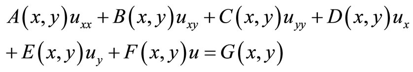
Let the second-order partial differential equation be in the form [1,2]
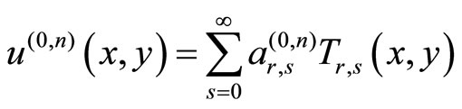
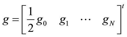
We assume that it has a Chebyshev series solution in the form
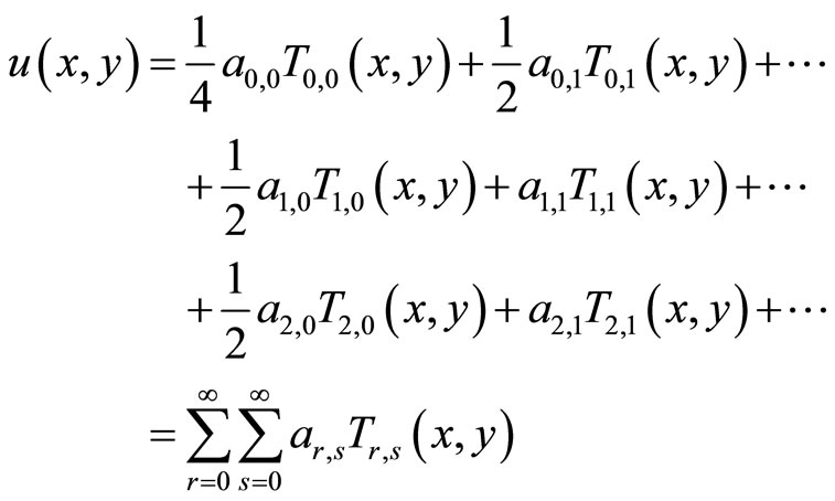 (1.2)
(1.2)
where  denotes a sum whose first term is halved. The unknown coefficients

 can be determined by using so called Chebyshev matrix method.
2. Calculation of Chebyshev Coefficients
Let we have a function ,
,  and its nth derivatives with respect to x can be expanded in Chebyshev series
and
Respectively, where  and
and  are Chebyshev coefficients; clearly,
  and
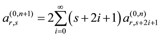
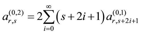
and  . Then the recurrence relation between the coefficients of
 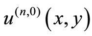 and
and 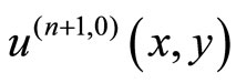 is obtained as
 (2.1)
(2.1)
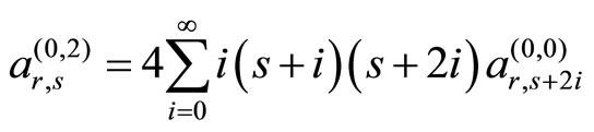
From Equation (2.1), we can deduce the relations
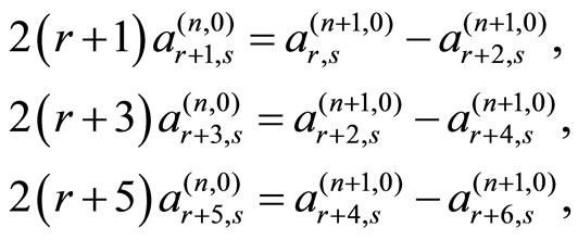
And adding these side by side, we get

or
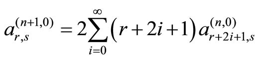 (2.2)
(2.2)
Specially, we can express the coefficients  and
and  in terms of the
  by means of Equation (2.2), in the forms
 (2.3)
(2.3)
and
or
 (2.4)
(2.4)
Now, let us take  and assume
  for
for ; then the system (2.2) can be transformed into the matrix form,
 (2.5)
(2.5)
where M is given in [3].
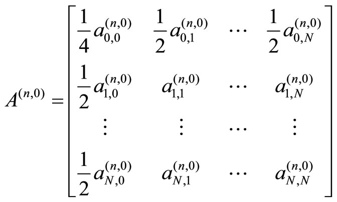
For  it follows from Equation (2.5) that
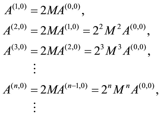 (2.6)
(2.6)
where clearly .
.
Let us assume, in the range , that the nth derivatives of
  with respect to y can be expanded in Chebyshev series
Respectively, where  and
and  are Chebyshev coefficients; clearly
  and
and  . Then the recurrence relation between the coefficients of
  and
and  is obtained as
 (2.7)
(2.7)
From Equation (2.7), we can deduce the relations

and adding these side by side, we get

or
 (2.8)
(2.8)
Specially, we can express the coefficients  and
and  in terms of the
 , by means of Equation (2.8), in the forms
 (2.9)
(2.9)
and
or
 (2.10)
Now, let us take  and assume
 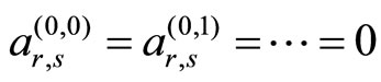 for
for ; then the system (2.8) can be transformed into the matrix form,
 (2.11)
where

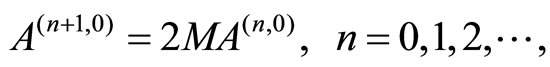
For 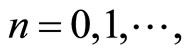 it follows from Equation (2.11) that
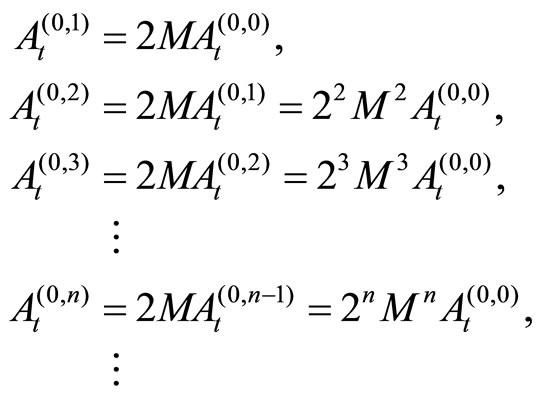 (2.12)
where clearly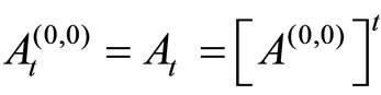 . Furthermore,
  can be expressed as follows:
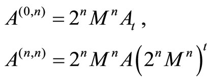 (2.13)
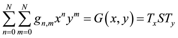
3. Fundamental Relations
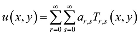
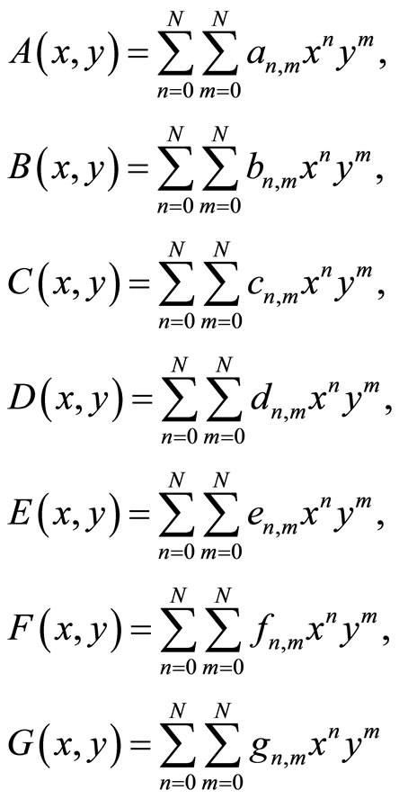
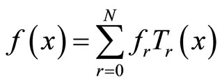
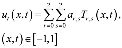
Now consider Equation (1.1), where A, B, C, D, E, F and G are functions of x and y, or constant, defined in the range . Our purpose is to investigate the truncated Chebyshev series solution of Equation (1.1), under the given conditions, in the series form
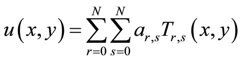
or in the matrix form
 (3.1)
(3.1)
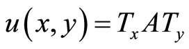
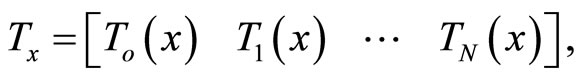
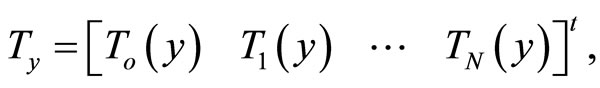
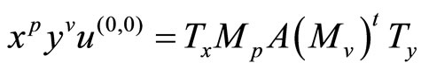
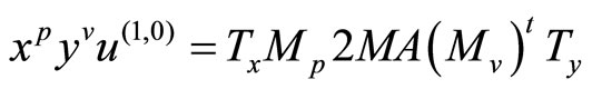
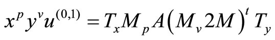
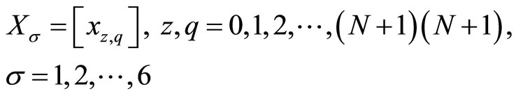
where ,
, 
 are the Chebyshev coefficients to be determined
  are the bivariate Chebyshev polynomials defined in [4], and matrices
 ,
,  and A are defined by

To obtain the solution of Equation (1.1) in the form of Equation (3.1), first we must reduce Equation (1.1) to a differential Equation whose coefficients are polynomials [5]. For this purpose, we assume that the functions ,
,  ,
,  ,
,  ,
,  ,
,  , and
, and  can be expressed in the form
 (3.2)
(3.2)
Which are Taylor polynomials at . By using the expressions (3.2) in Equation (1.1), we get
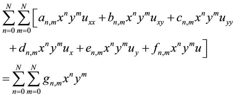 (3.3)
(3.3)
The Chebyshev expansions of terms

in Equation (3.3) are obtained by means of the formulae
 (3.4)
(3.4)
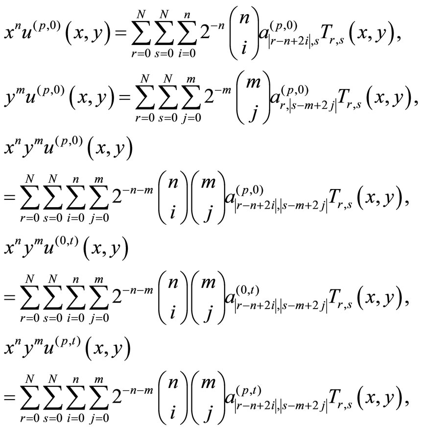
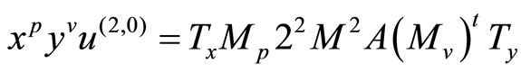
4. Matrix Forms of Terms in the Equation
The matrix representation of Equation (3.4) can be given by
 (4.1)
(4.1)
 (4.2)
(4.2)
 (4.3)
(4.3)
 (4.4)
(4.4)
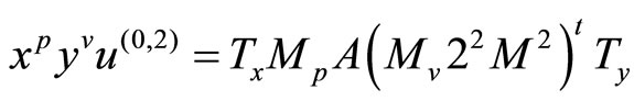 (4.5)
(4.5)
 (4.6)
(4.6)
 (4.7)
(4.7)
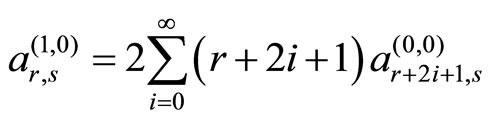
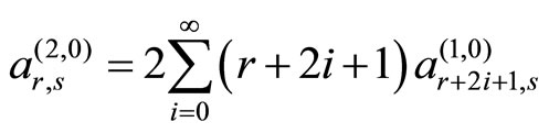
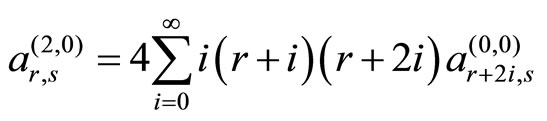
where 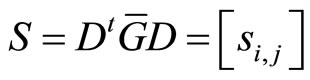 and
and ,
,  .
.
And for ;
; ,
,  (
( and
and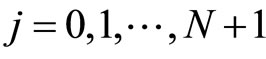 ) is a matrix of size
 . The elements of Mp are given in [6].
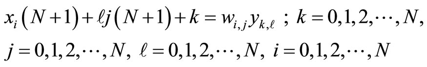
Substituting the expressions (4.1)-(4.7) into Equation (3.3), and simplifying the result, we have the matrix equation
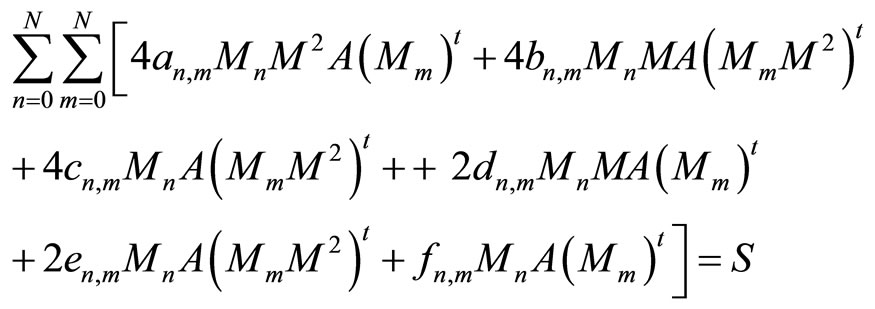 (4.8)
(4.8)
Which corresponds to a system  algebraic equations for the unknown Chebyshev coefficients
 . Briefly, we can assume that Equation (4.8) is given in the form
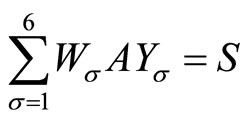 (4.9)
(4.9)
where 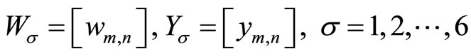
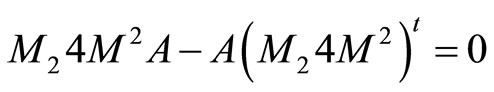
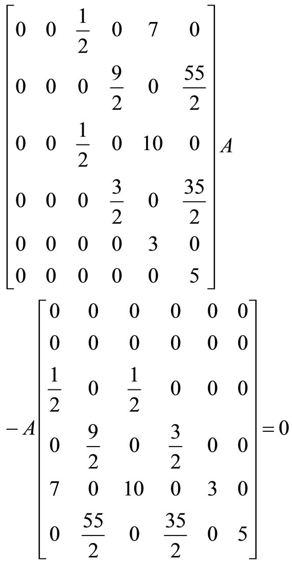
Matrix Equation (4.9) can be reduce to new matrix equation by making use of
Then the new matrix Equation (4.7) becomes
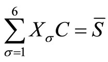 (4.10)
where
and


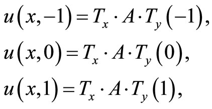
5. Matrix Forms of Conditions
Let the conditions of Equation (1.1) be given by
 (5.1)
(5.1)
 (5.2)
(5.2)
 (5.3)
(5.3)
where f is a function of x, g is a function of y and  is constant.
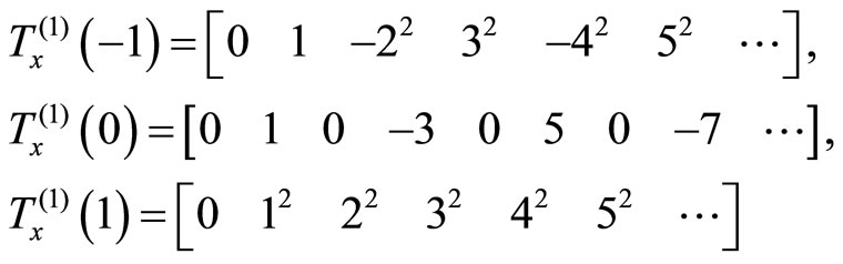
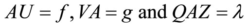
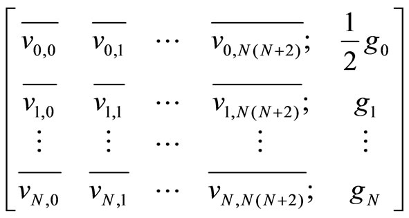
Then, there are the following matrix forms at x = −1, 0, 1 and similar way for y = −1, 0, 1;
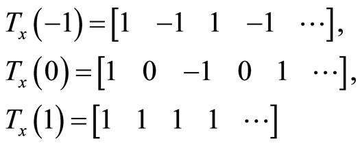
Derivative of Tx at x = −1, 0, 1 and similar way for y = −1, 0, 1;
We assume that the functions  and
and  can be expanded as
and

or in the matrix form
and
where

In addition, at x = −1, 0, 1 and y = −1, 0, 1, we obtain the matrix forms
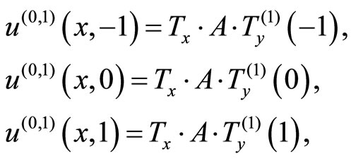
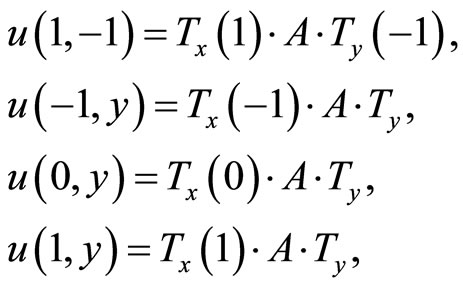
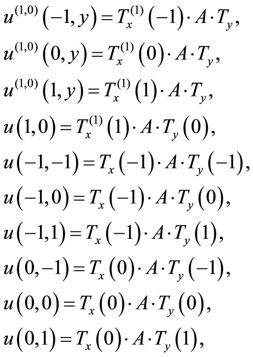
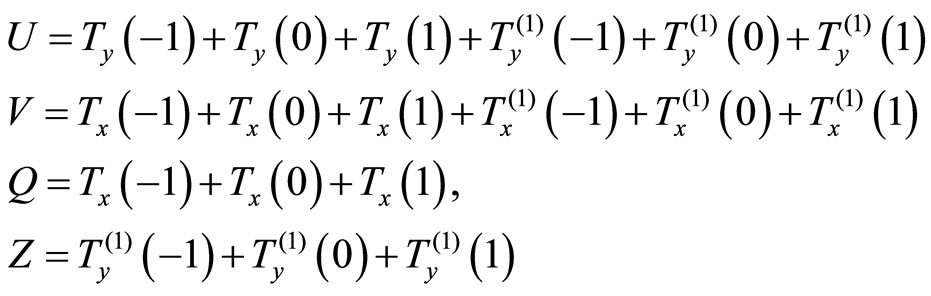
Substituting theses matrices forms into conditions (5.1)-(5.3), and then simplifying, we get the fundamental matrix equations of conditions as follows:
 (5.4)
(5.4)
where
6. Former Method for the Solution
We can assume that Equation (6.1) is in the form
 (6.1)
(6.1)
where .
.
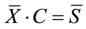
Then the augmented matrix of Equation (6.1) becomes  or
or
 (6.2)
(6.2)
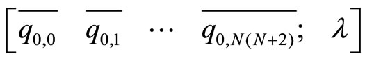
If we take the new matrix forms of the conditions as ,
,  and
and , respectively, the augmented matrices of them become
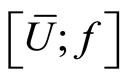 ,
, 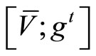 and
and 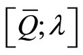 or more clearly
 (6.3)
(6.3)
 (6.4)
(6.4)
and
 (6.5)
(6.5)
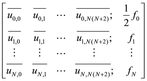
Consequently, by replacing Equations (6.3)-(6.5) by the last 2N + 1 rows of Equation (6.2), we have the new augment matrix
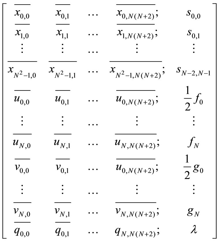
From the solution of this system we can find matrix C or matrix A.
7. Applications
The Chebyshev matrix method applied in this study is useful in finding approximate solutions of second-order linear partial differential equations in both homogeneous and non-homogeneous cases, in terms of Chebyshev polynomials. We illustrate it by the following examples.
Example 1. We now consider the problem [7]:
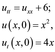 (1)
(1)
And seek the solution in the form
 (2)
(2)
Then we obtain the matrix equation
 (3)
(3)
where
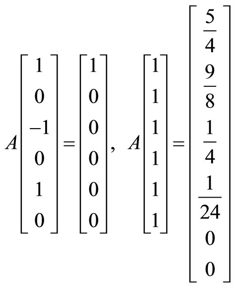
And the condition matrices are
 (4)
(4)
 (5)
(5)
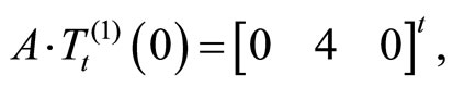
By replacing the new matrix form of Equations (4) and (5) in the new matrix form of Equation (3), we have the matrix equation under given conditions as follows:
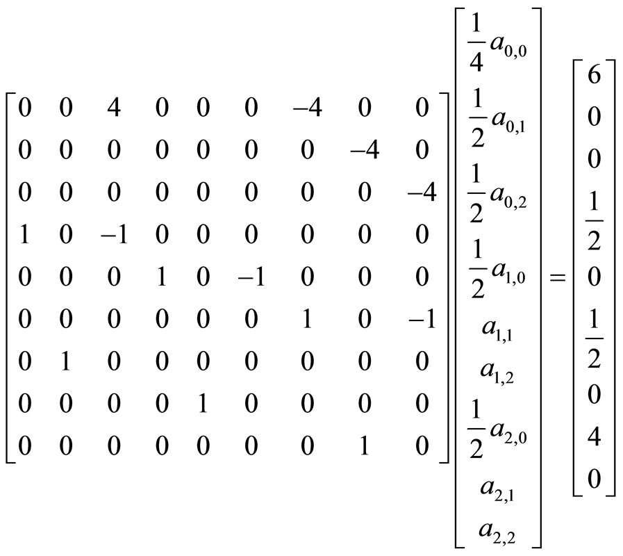
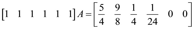
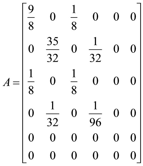
Hence, we obtain the augmented matrix
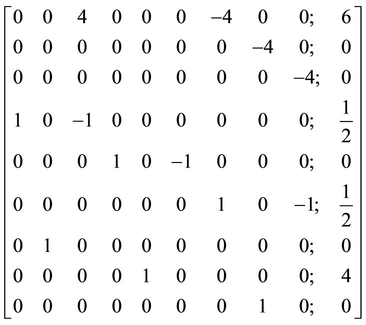
The solution of this system is
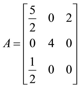
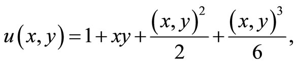
and thereby the solution of the problem (1) becomes
or

This is exact solution [7].
Example 2
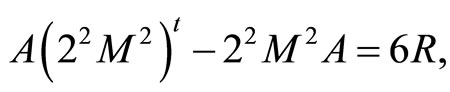
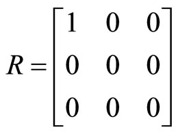
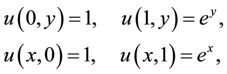
Let us now study the equation
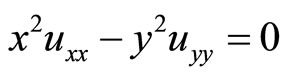
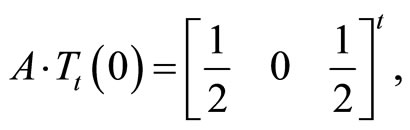
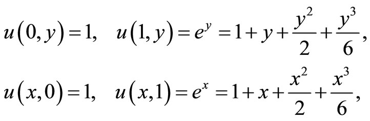
with conditions which are
The first four terms of the series expansions:
Chebyshev matrix forms of the conditions,

Matrix form of the equation is
From the solution of this matrix equation under the given conditions, we get the Chebyshev coefficients matrix as
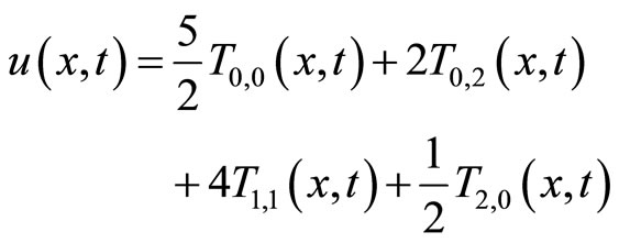
The solution of problem is obtained as
Which is the first four terms of .
.
8. Conclusions
Analytic solutions of the second order linear partial differential equations with variable coefficients are usually difficult. In many cases, it is required to approximate solutions. For this purpose, the Chebyshev matrix method can be proposed.
In this study, the usefulness of the Chebyshev matrix method presented for the approximate solution of the second order linear partial differential equations is discussed. Also, the method can be applied to both the nonhomogeneous and homogeneous cases.
A considerable advantage of the method is that the solution is expressed as a truncated Chebyshev series and thereby a Taylor polynomial. Furthermore, after calculation of the series coefficients, the solution  of the equations can be easily evaluated for arbitrary values of
  at low computation effort.
An interesting feature of the Chebyshev matrix method is that the method can be used in finding exact solutions in much cases. The method can be also extending to the solution of the higher order linear partial differential equations.
REFERENCES
- X. F. Yang, Y. X. Liu and S. Bai, “A Numerical Solution of Second-Order Linear Partial Differential Equations by Differential Transform,” Journal of Applied Mathematics and Computing, Vol. 173, No. 2, 2006, pp. 792-802. doi:10.1016/j.amc.2005.04.015
- L. H. Ye and Z. T. Xu, “Oscillation Criteria for Second Order Quasilinear Neutral Delay Differential Equations,” Journal of Applied Mathematics and Computing, Vol. 207, No. 2, 2009, pp. 388-396. doi:10.1016/j.amc.2008.10.051
- M. Sezer and M. Kaynak, “Chebyshev Polynomial Solutions of Linear Differential Equations,” International Journal of Mathematical Education in Science & Technology, Vol. 27, No. 4, 1996, pp. 607-618. doi:10.1080/0020739960270414
- N. K. Basu, “On Double Chebyshev Series Approximation,” SIAM Journal on Numerical Analysis, Vol. 10, No. 3, 1973, pp. 496-505. doi:10.1137/0710045
- F. Cases, “Solution of Linear Partial Differential Equations by Lie Algebraic Methods,” Journal of Computational and Applied Mathematics, Vol. 76, No. 1-2, 1996, pp. 159-170.
- H. Koroglu, “Chebyshev Series Solution of Linear Fredholm Integrodifferential Equations,” International Journal of Mathematical Education in Science & Technology, Vol. 29, No. 4, 1998, pp. 489-500. doi:10.1080/0020739980290403
- V. S. Vladimirov, “A Collection of Problems on the Equations of Mathematical Physics,” Mir Publishers, Moscow, 1986, pp. 139-149.