Applied Mathematics
Vol. 3 No. 11A (2012) , Article ID: 24758 , 7 pages DOI:10.4236/am.2012.331246
Investigation of Effects of Large Dielectric Constants on Triaxial Induction Logs
Electrical Engineering Department, University of Housotn, Houston, USA
Email: zzhijuan@yahoo.com
Received August 6, 2012; revised September 6, 2012; accepted September 13, 2012
Keywords: Resistivity; Dielectric; Simulation; Interpretation
ABSTRACT
The dielectric effect is receiving increasing interest in the study of resistivity logging. Several recent findings have proven that the dielectric effect can cause negative imaginary signals on the array induction logging. However, very few researches discuss the dielectric effect on the triaxial induction logging which is a novel technology in solving anisotropy problem. In this paper, we investigate the effect of large dielectric constants on a basic triaxial induction tool in a 1-D homogenous earth formation. The simulation model is derived from Maxwell equation and calculated by wave number integration. Sufficient simulations have been done. We performed an asymptotic analysis of the dielectric effect within the low-freq limit, yielding interesting observations on the dielectric effect with respect to frequency, spacing, and anisotropy. Those findings provide important and useful guidance for researchers to study on the dielectric effect on the triaxial induction logging.
1. Introduction
Plentiful experiments have shown that at a low frequency, dielectric constants are significantly increased. For instance, Sengwa-Soni showed that the relative dielectric permittivity, εr, of water-saturated carbonate could be higher than 1000 when its frequency is at 100 Hz [1]; Ahualli discovered that in the highly concentrated colloidal fluid, εr could be more than 1000 at the frequency of 300 Hz [2]. Specifically, the dielectric constant can reach up to 50,000 in shale formations with metallic particles at an induction frequency range of (25 - 100 KHz) [3].
The reason is very complex and still under study since dielectric enhancement violates the equal distribution principle. The most common explanation is a double electric layer model [4]. A new rock model that simulates conductive grain enclosed by a super thin, non-conductive coating was found to be effective in explaining dielectric enhancement in rocks [5]. It is the low-conductivity membrane that causes dielectric enhancement at low frequencies in rock formations.
Induction logging tools operating at a low frequency (10 KHz - 400 KHz) is one important approach to detect the resistivity of the earth formations. In the induction operation range, the dielectric effect is negligible within the range of typical formation conductivities (0.5 - 5 S/m), because the displacement current is relatively smaller than the conduction current. However, in the recent years within the current decade, strange induction logs with large negative imaginary signals (also called as X-signals) in array induction logs have been encountered and successfully explained by large dielectric constants (εr > 10,000) [6,7].
Responses from traditional array induction logging are essentially coaxial components which transmitters and receivers are placed along the same axis. Because of the structure limitation, the traditional induction tool is not able to detect anisotropy. Advanced induction technology has been developed and is known as a triaxial induction tool. It is comprised by three mutually perpendicular pairs of transmitters and receivers and capable to collect multi-directional electrical information. Responses on a triaxial tool can be categorized into three aspects: coaxial, coplanar, and cross components. In fact, the coplanar responses play an important role in determining anisotropic resistivity. Some cross components give contributions to detect formation boundary. The inversion approach has been developed to detect dipping angle based on both coplanar and cross components [8-11]. However, the dielectric effect on coplanar and cross components is still unknown. Hence it is worthy to investigate the dielectric enhancement effect on those components, based on the structure of triaxial induction logging tool. The purpose of this paper is to discuss the effect of large dialectic constants on a triaxial induction logging tool. A 1-D synthetic model of a triaxial tool in homogenous transverse isotropic (TI) formation at an arbitrary dipping angle is employed to simulate the dielectric effect on triaxial responses. An asymptotic analysis approach is implemented to investigate dielectric effect.
2. 1-D Modeling
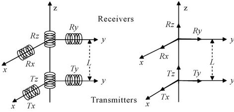
A basic structure of the triaxial induction tool consists of three orthogonal transmitters and three orthogonal receivers oriented at x, y, and z direction, as shown in Figure 1(a). Since the transmitter and receiver coils are infinitely small, we can treat them as magnetic dipoles. The equivalent dipole model is shown in Figure 1(b). For industry standard wire line triaxial tools, bucking coils placed between the transmitters and the receivers are always implemented to eliminate the direct coupling radiated from the transmitters.
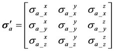
A 3 × 3 tensor apparent conductivities  is measured at each pair of transmitter-receiver spacing,
 (1)
(1)
 (2)
(2)
where  is the measured apparent conductivity at the j-th receiver from the i-th transmitter.
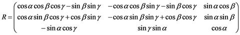
Consider a triaxial tool in a 1-D TI medium. The orientation of transmitter and receiver is arbitrary with respect to formation coordinate. Figure 2 shows two types of coordinates in the whole system: the formation coordinates (unprimed) and the sonde coordinate (primed). The symbol α is a dipping angle between the Z axis and the  axis. The symbol β is an azimuthal angle between the x axis and the projection of transmitter coils on the X-Y plane. The symbol γ represents a rotation angle that transmitter Tx is deviated from the
  axis.
axis.
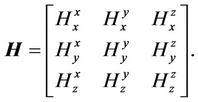
The transformation of magnitudes between the bedding-plane coordinates X, Y, Z and the tool-system coordinates ,
,  , and
, and  is affected by the same rotation matrix as We assume that
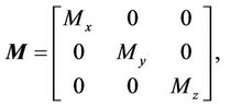
  denotes the magnetic moment in the sonde coordinate, given by
 (3)
(3)
Then in the formation coordinate, the equivalent magnetic source M is obtained by
 (4)
(4)
In the formation coordinate, Maxwell equations due to
 (a) (b)
Figure 1. Basic structure of a triaxial induction tool [12]. (a) The original model; (b) The equivalent model.
a magnetic source M are shown as,
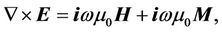 (5)
(5)
and
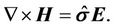 (6)
(6)
where , M,
, M,  are defined as
 (7)
(7)
 (8)
(8)
 (9)
(9)
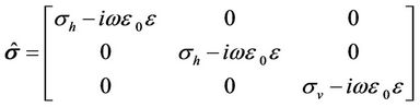
Note that the dielectric permittivity  and electric conductivity tensor
  are combined into a single, complex-valued conductivity
 . In terms of Equations (5) and (6), we can analytically solve magnetic fields in a homogenous formation. The details of the derivation are omitted here and can be referred to [13].
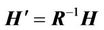
Magnetic responses in the sonde system is easily derived by multiplying the inverse of rotation matrix to magnetic components in formation coordinate, as
 (10)
(10)
where  is the magnetic filed is defined as
 (11)
(11)
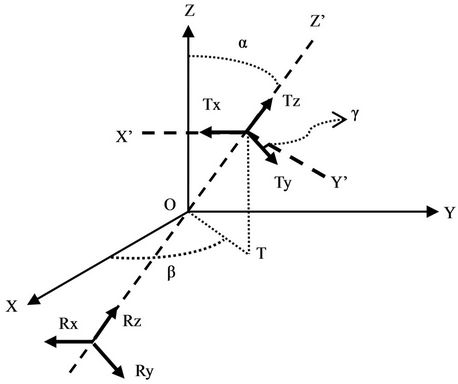
Figure 2. The relationship between tool coordinate and formation coordinate.
The magnetic fields in Equation (11) are consisted by direct coupling and the induced secondary fields. The latter one is dominated by the conductivity of the formation and always overwhelmed by the direct coupling. As we mentioned before, bucking coils are implemented to distract direct coupling from the total fields and leave the secondary fields. We can adjust the distance, turns or windings of the bucking coils to balance off direct fields. In this paper, we take use of spacing to eliminate direct coupling [10], shown as
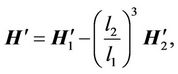 (12)
(12)
where  is the final magnetic filed and l1, l2 are distance to bucking coil and main receiver.
Finally we can find the apparent conductivity tensor  with respect to Equation (12), as
 (13)
(13)
K is the conversion matrix given by tool specific configuration [12], shown as,
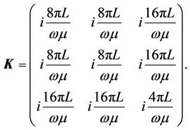 (14)
(14)
Specifically, if the well is vertical, the apparent conductivity tensor  would be a diagonal matrix, as
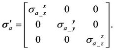 (15)
(15)
In Equation (15), 
 are coplanar components. In TI medium,
  and
and  are the same as each other because of the symmetric resistivity in horizontal plane. Thus in the following part, we only need to discuss
 .
.  is basically the coaxial response, which is the same as from an array induction tool.
In the deviated well, the apparent conductivity tensor  is given by
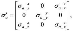 (16)
(16)
with two nonzero cross components 
 due to nonzero dipping angle. It is found that the horn effect on
  and
and  is an important indicator of formation boundary.
3. Results and Discussion
3.1. Example 1
In the first example, we assume a homogenous isotropic formation, whose conductivity is 0.1 S/m. We set the tool movement trajectory perpendicular to formation, namely, zero dipping angle. The distance between transmitter and main receiver and bucking coil are 21 inch, 15 inch, respectively. Without specification, the same distance between transmitter and main receiver and bucking coil are the same as in the first example.
3.1.1 Case I: f = 26 KHz, 52 KHz, 104 KHz
In Figure 3, we present coplanar component  and coaxial component
  versus permittivity
  (1 - 50,000) at 26 KHz, 52 KHz and 104 KHz, respectively.
Simulation results in Figure 3 reveal that dielectric enhancement does take effect on apparent conductivity  and
and . X-signals of both apparent conductivities
  and
and  are decreased and become negative at higher permittivity
 . Meanwhile, R-signal increases significantly with the increased permittivity
 . Therefore, we predict dielectric enhancement can also cause negative sign on the imaginary components of apparent conductivity
  and
and  whereas the real components are positively enhanced.
Then in Table 1, we summarize the minimum values of permittivity  that induce 10% discrepancy on apparent conductivity
  and
and  with and without dielectric enhancement. Specifically, we name those dielectric constants as effective dielectric constants.
According to Table 1, effective dielectric constants on the real parts of apparent conductivity  and
and  are reverse proportional to frequency. Therefore, we infer that higher frequency manifests dielectric effect, which obeys the definition of the complex conductivity
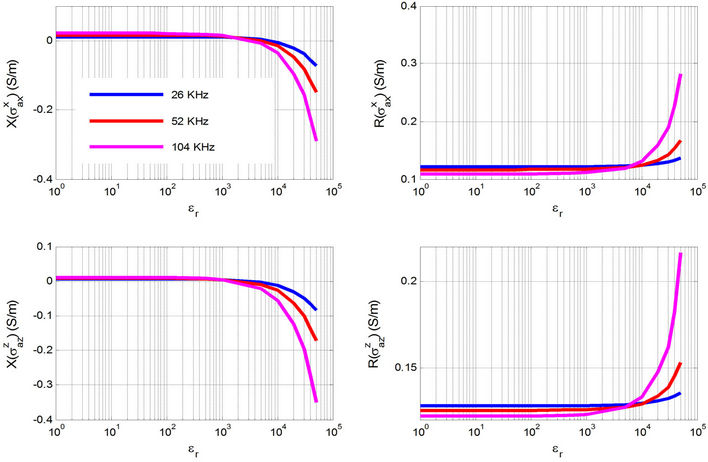
Figure 3. Rand X-components of apparent conductivities  and
and  with respect to the relative permittivity
 .
.
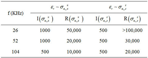
Table 1. List of effective dielectric constants inducing 10% discrepancy on apparent conductivity  and
and  with and without dielectric enhancement.
given by Equation (8). The abnormally large dielectric constant is frequency dependent. Thus smaller dielectric constants are in need to reach the same level dielectric effect.
On the other hand, the effective dielectric constants on X-signal of apparent conductivity  and
and  are much smaller than on R-signal. Thus we know that imaginary components are more sensitive to dielectric effect than the real parts.
3.1.2 Case II: 
Secondly, we investigate the relationship between coil spacing and the dielectric effect with the same isotropic formation. Table 2 lists the corresponding coil spacing between transmitter and main receiver and bucking coils.
Figure 4 compares Rand X-components of apparent conductivities  and
and  with respect to the coil spacing for small permittivity (
 ) and large dielectric constant (
 ), respectively. A significant nonlinear discrepancy on X-signals with and without large permittivity is shown and changed into negative
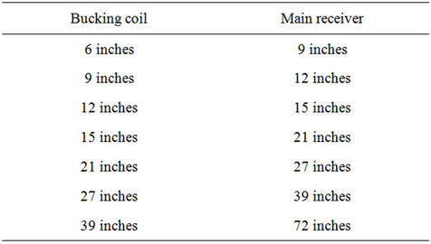
Table 2. List of coil spacing from the transmitter to main receiver and bucking coil.
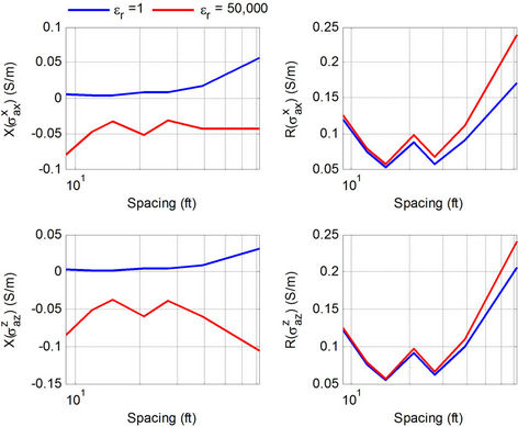
Figure 4. Rand X-components of apparent conductivities  and
and  with respect to coil spacing. The conductivity is 0.1 S/m. The frequency is 26 KHz.
signs.
3.2. Example 2
In this example, we consider a TI formation and figure out dielectric enhancement on anisotropic conductivity in layered laminated formation. The frequency is 26 KHz.
3.2.1. Case I: 
Vertical conductivity  is assumed as 0.1 S/m and horizontal conductivity
  is changing from 0.1 S/m to 10 S/m. The simulation results of coplanar component
  with respect to horizontal conductivity
  are presented in Figure 5.
In Figure 5, the x axis is the anisotropic ratio . As shown in Figure 5, weak discrepancy on the apparent conductivities
  and
and  with and without the dielectric effect is observed. In order to illustrate explicitly, we present relative error
  in Figure 6.
Figure 6. shows that with the increased horizontal conductivity , dielectric effect on both X-and R-
 and
and  is decreased. According to the conductive property of laminated anisotropic medium, the horizontal conductivity
  is dominated by salt water zone for laminated formation and thus we can infer that dielectric effect on
 ,
,  may be attenuated in the water-bearing zone.
3.2.2. Case II: 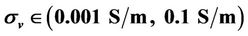
Next, we restore the horizontal conductivity  to be
to be
Figure 5. Rand X-components of apparent conductivities  and
and  with respect to anisotropic ratio
 . The vertical conductivity
  is a constant and set as 0.1 S/m. The horizontal conductivity
  is various from 0.1 S/m to 1 S/m. The frequency is 26 KHz.
Figure 6. The relative error  of apparent conductivities
  and
and  with and without dielectric enhancement.
0.1 S/m and alter vertical conductivity  from 0.001 S/m to 0.1 S/m. Figure 7 compares apparent conductivities
  and
and  with and without dielectric effect in a similar way as shown in Figure 6. In this example, the distance from the transmitter to the main receiver and bucking coil are 21 inch, 15 inch, respectively.
Since the horizontal conductivity  is constant, Rand X-
 are independent to the vertical conductivity. Thus we know the discrepancy of the coaxial component
  is only related to dielectric effect. We have observed that X-
 is negative when
  is 50,000, which is caused by large vertical permittivity.
Figure 8 presents the absolute relative differences 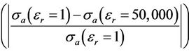 of apparent components
 with and without the dielectric effect, respectively. With larger anisotropic ratio, the relative differences on Xand R-
 are increasing. In the laminated anisotropic medium, the vertical conductivity is dominated by a hydrocarbon zone, and we can conclude that dielectric effect on
 would be boosted by the hydrocarbon-bearing zone.
3.3. Example 3
Cross components 
 are helpful for detecting the formation boundary; therefore, efficiently help us solve multilayer inversion problem. Hence in this section, we will discuss how the dielectric effect takes effect in the deviated well.
We now assume one homogenous anisotropic medium, whose anisotropic ratio is 10 (σh = 1 S/m, σv = 0.1 S/m).
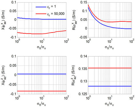
Figure 7. Rand X-components of both  and
and  with respect to anisotropic ratio
 . The vertical conductivity
  is various. The horizontal conductivity
  is 0.1 S/m. The frequency is 26 KHz.
Figure 8. The absolute relative difference  of Rand X-components of both
  and
and  when
when  or 50,000, respectively, with respect to anisotropic ratio
 .
.
The frequency is 26 KHz. Figure 9 shows off-diagonal apparent responses, 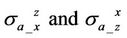 , with respect to dipping angle α.
The R-signal of  and
and  from normal and large permittivities are perfectly coincide with each other; and therefore, R-signal of both
  and
and  are independent with dielectric effect in any deviated well. We observe one interesting phenomenon in the X-signals of both
  and
and . If the well is slightly deviated (α ≤ 10˚) or highly deviated (α ≥ 85˚), the discrepancy on
Figure 9. Rand Xcomponents of  and
and  with respect to the dipping angle, α. The horizontal conductivity
  and the vertical conductivity
  are 1 S/m, and 0.1 S/m, respectively. The frequency is 26 KHz. The distance from the transmitter to the main receiver and bucking coil are 21inches, 15inches, respectively.
X-signal of  and
and  is negligible. However, in the medium range (10˚ < α < 85˚), X-signal of
  or
or  with
with  is differentiated from small permittivity (
 ). Thus we can infer that in a vertical or highly deviated borehole, the dielectric effect can be ignored on the cross components,
 during inversion, even though large dielectric constants do exist.
4. Conclusions
Previous work has proven that the dielectric effect causes the negative X-signal of array induction logging. We extend this discussion to triaxial induction logs and discuss the dielectric effect on the coplanar, coaxial, and cross components.
A 1-D synthetic forward model for the triaxial induction tool in the homogenous medium is explained and implemented. We employ the triaxial tool includes bucking coils to eliminate direct coupling between the transmitters and main receivers.
Sets of asymptotic analysis are illustrated. We find that the dielectric effect may cause negative signs on the imaginary components of both coplanar and coaxial responses of triaxial induction logs and enhance the real component. The dielectric effect is enhanced by high operation frequency as well as long coil spacing.
In the laminated anisotropic medium, the hydrocarbon-bearing zone manifests the dielectric effect, whereas the water-bearing zone weakens the dielectric effect. Additionally, the dielectric effect plays a negligible impact on the cross components, 
 for vertical or highly deviated well.
5. Acknowledgements
The authors are indebted to the Well Logging Laboratory for their kind permission to provide the forward model code.
REFERENCES
- R. J. Sengwa and A. Soni, “Low-Frequency Dielectric Dispersion and Microwave Dielectric Properties of Dry and Water-Saturated Limestones of the Jodhpur Region,” Geophysics, Vol. 71, No. 5, 2006, pp. G269-G277. doi:10.1190/1.2243743
- S. Ahualli, M. L. Jiménez and A. V. Delgado, “Electroacoustic and Dielectric Dispersion of Concentrated Colloidal Suspensions,” IEEE Transactions on Dielectrics and Electrical Insulation, Vol. 13, No. 3, 2006, pp. 657-663. doi:10.1109/TDEI.2006.1657981
- R. H. Hardman and L. C. Shen, “Theory of Induction Sonde in Dipping Beds,” Geophysics, Vol. 51, No. 3, 1986, pp. 800-809. doi:10.1190/1.1442132
- M. B. McBRIDE, “A Critical of Diffuse Double Layer Models Applied to Colloid and Surface Chemistry,” Clays and Clay Minerals, Vol. 45, No. 4, 1997, pp. 598-608.
- M. Luo and C. Liu, “Numerical Simulations of Large Dielectric Enhancement in Some Rocks,” Society of Geophysical Exploration, CPS/SEG Beijing 2009 Conference and Exposition, Beijing, 2009.
- B. Anderson, T. Barber, and M. Luling, “Observations of Large Dielectric Effects on Induction Logs, or Can Source Rocks Be Detected with Induction Measurements,” Society of Professional Well Log Analysts Publications, Symposium Transactions, Veracruz, 4-7 June 2006.
- B. Anderson, T. Barber, M. Luling, J. Rasmus and P. Sen, “Observations of Large Dielectric Effects on LWD Propagation-Resistivity Logs,” Symposium Transactions on Society of Professional Well Log Analysts Publications, Austin, 3-6 June 2007.
- Z. Zhang, L. Yu, B. Kriegshauser and L. Tabarovasky, “Determination of Relative Angles and Anisotropic Resistivity Using Multicomponent Induction Logging Data,” Geophysics, Vol. 69, No. 4, 2004, pp. 898-908. doi:10.1190/1.1778233
- B. I. Anderson, T. D. Barber and T. M. Habashy, “The Interpretation and Inversion of Fully Triaxial Induction Data: A Sensitivity Study,” Transactions of the SPWLA 25th Annual Logging Symposium, Oiso, 1-13 June 2002.
- B. Krieghauser, O. Fanini, S. Forgang, G. Itskovich, M. Rabinovich, L. Tabarovsy, L. Yu, M. Epov, P. Gupta and J. V. D. Horst, “A New Multicomponent Induction Logging Tool to Resolve Anisotropic Formations,” Transactions SPWLA 41st Annual Logging Symposium, Dallas, 4-7 June 2000.
- G. S. Liu, F. L. Teixeira and G. J. Zhang, “Analysis of Directional Logging Sensors,” IEEE Transactions on Geoscience and Remote Sensing, Vol. 48, No. 3, 2010, pp. 1151-1158.
- J. H. Moran and K. S. Kunz, “Basic Theory of Induction Logging and Application to Study of Two-Coil Sondes,” Geophysics, Vol. 27, No. 6, 1962, pp. 829-858. doi:10.1190/1.1439108
- L. Zhong, J. Li, A. Bhardwaj, L. C. Shen and R. C. Liu, “Computation of Triaxial Induction Logging Tools in Layered Anisotropic Dipping Formations,” IEEE Transactions on Geoscience and Remote Sensing, Vol. 46, No. 4, 2008, pp. 1148-1163. doi:10.1109/TGRS.2008.915749