Applied Mathematics
Vol.3 No.8(2012), Article ID:21479,9 pages DOI:10.4236/am.2012.38128
Modified Fletcher-Reeves and Dai-Yuan Conjugate Gradient Methods for Solving Optimal Control Problem of Monodomain Model
Department of Mathematical Sciences, Faculty of Science, Universiti Teknologi Malaysia, Johor Bahru, Malaysia
Email: kwng3@live.utm.my, rohanin@utm.my
Received May 17, 2012; revised June 17, 2012; accepted June 24, 2012
Keywords: Monodomain Model; Conjugate Gradient Method; Galerkin Finite Element Method; Optimal Control
ABSTRACT
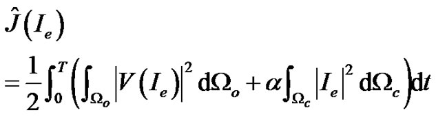
In this paper, we present the numerical solution for the optimal control problem of monodomain model with Rogersmodified FitzHugh-Nagumo ion kinetic. The monodomain model, which is a well-known mathematical model for simulation of cardiac electrical activity, appears as the constraint in our problem. Our control objective is to dampen the excitation wavefront of the transmembrane potential in the observation domain using optimal applied current. Various conjugate gradient methods have been applied by researchers for solving this type of optimal control problem. For the present paper, we adopt the modified Fletcher-Reeves method and modified Dai-Yuan method for computing the optimal applied current. Numerical results show that the excitation wavefront is successfully dampened out by the optimal applied current when the modified Fletcher-Reeves method is used. However, this is not the case when the modified Dai-Yuan method is employed. Numerical results indicate that the modified Dai-Yuan method failed to converge to the optimal solution when the Armijo line search is used.
1. Introduction
Sudden cardiac death is a leading cause of death among adults in most countries. In the United States, sudden cardiac death episodes affect 450,000 people each year [1]. In Singapore, about 23% of approximately 16,000 deaths that occur every year are reported as cardiac death [2]. Also, a recent study in China indicates that sudden cardiac death takes the lives of over 544,000 people annually [3]. Sudden cardiac death occurs when the electrical system of the heart malfunctions, causing an irregular heart rhythm. This irregular heart rhythm cause the heart muscle to quiver and the heart is no longer able to pump blood to the body and brain. Consequently, death can occurs within minutes unless the normal heart rhythm is restored through defibrillation. Nowadays, the implantable cardioverter defibrillator (ICD) is increasingly being used by patients who are at significant risk of sudden cardiac death. If any life-threatening arrhythmia is detected by ICD, an energy electrical shock will be delivered to the heart to restore normal heart rhythm.
The optimal control approach to the defibrillation process was first proposed by Nagaiah et al. [4], with the objective to determine the minimal applied current which can help in the defibrillation process. More specifically, the control objective is to dampen the excitation wavefront of the transmembrane potential in the observation domain using optimal applied current. The monodomain model was employed by Nagaiah et al. [4] to represent the electrical behavior of the cardiac tissue. The monodomain model consists of a parabolic partial differential equation (PDE) coupled to a system of nonlinear ordinary differential equations (ODEs), which is a wellknown mathematical model for simulation of cardiac electrical activity [5-7]. Consequently, the optimization problem of defibrillation process can be generally known as optimal control problem of monodomain model.
In the literature, the nonlinear conjugate gradient methods have been frequently applied by researchers for solving the optimal control problem of the monodomain model. Nagaiah et al. [4] employed the Polak-RibièrePolyak (PRP) method [8,9], the Hager-Zhang (HZ) method [10] and the Dai-Yuan (DY) method [11] to solve the optimal control problem of this monodomain model. Later, Ng and Rohanin [12] utilized the modified version of the DY method as proposed by Zhang [13] to solve the optimal control problem of monodomain model. On the other hand, the Hestenes-Stiefel (HS) method [14] has been applied by Ainseba et al. [15] for solving the optimal control problem of tridomain model. For the present paper, we present the numerical solution for the optimal control problem of monodomain model using two modified conjugate gradient methods, namely modified Fletcher-Reeves (MFR) method [16] and modified Dai-Yuan (MDY) method [17].
This paper is organized as follows: In Section 2, we present the optimal control problem of monodomain model with Rogers-modified FitzHugh-Nagumo ion kinetic. In Section 3, we discuss the optimize-then-discretize approach used to discretize the optimal control problem. In Section 4, we present the optimization procedure for solving the discretized optimal control problem. Next, the numerical experiment results are given in Section 5. Lastly, we conclude our paper in Section 6.
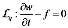
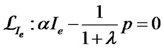
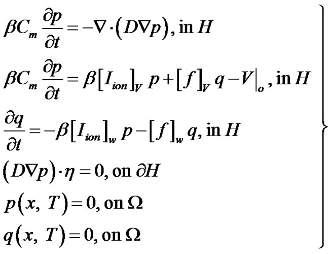
2. Optimal Control Problem of Monodomain Model
In this section, we present the optimal control problem of monodomain model with Rogers-modified FitzHughNagumo ion kinetic. Let  be the computational domain with Lipschitz boundary
 ,
,  be the observation domain and
  be the control domain. We further set
  and
and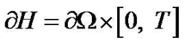 . The optimal control problem of monodomain model is therefore given by
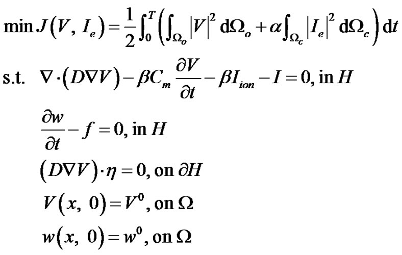 (1)
(1)
where
 (2)
(2)
 (3)
(3)
 (4)
(4)
Here  is the regularization parameter,
  is the final simulation time,
  is the outer normal to
 ,
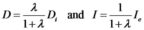
,  is the intracellular conductivity tensor,
  is the surface-to-volume ratio of the cell membrane,
  is the membrane capacitance,
  is the constant scalar used to relate the intracellular and extracellular conductivity tensors,
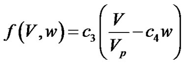
  is the plateau potential,
  is the threshold potential,
  are positive parameters,
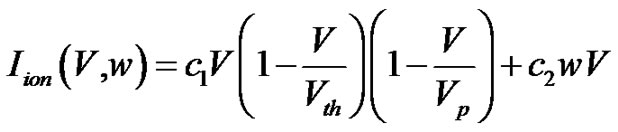
 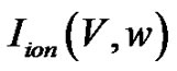 is the current density flowing through the ionic channels,
  is the prescribed vector-value function,
  is the transmembrane potential,
  is the extracellular current density stimulus and
  is the ionic current variable. Note that Equations (3) and (4) are obtained from the Rogers-modified FitzHugh-Nagumo model [18].
For the optimal control problem defined in Equation (1),  is the control variable while
  and
and  are the state variables. The control variable
  is chosen such that it is nontrivial only on
 , and extended by zero on
 . Furthermore,
  is chosen in the best possible way to achieve the control objective, i.e. to dampen out the excitation wavefront of transmembrane potential
  in the observation domain
 .
.
Kunisch and Wagner [19] proved that the controlto-state mapping is well-defined for the optimal control problem of monodomain model, i.e.
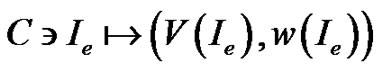 . This allows us to rewrite the cost functional in Equation (1) as
 (5)
(5)
where Equation (5) is known as the reduced cost functional.
3. Discretization of Optimal Control Problem
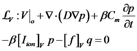
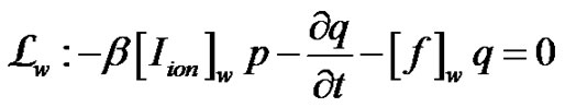
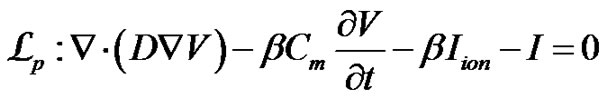
In the present paper, a classical approach is used to discretize the optimal control problem of monodomain model, i.e. the optimize-then-discretize approach. Let’s introduce the Lagrange multipliers 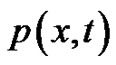 and
and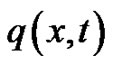 , which arealso known as the adjoint variables, the Lagrange functional
  is therefore defined as
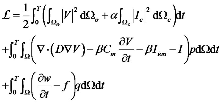 (6)
(6)
The first-order necessary conditions for optimality are stated by requiring stationarity of Equation (6) with respect to , resulting in
 (7)
(7)
 (8)
(8)
 (9)
(9)
 (10)
(10)
 (11)
(11)
where  denotes the partial derivative with respect to * and
  denotes the transmembrane potential in
 . We further obtain the terminal and boundary conditions as follows
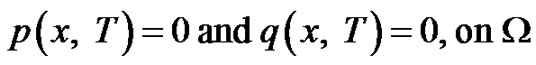 (12)
(12)
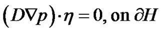 (13)
(13)
By utilizing the initial and boundary conditions in Equation (1) as well as Equations (7)-(13), the state and adjoint systems can be formed as follows
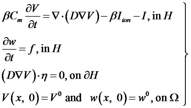 (14)
(14)
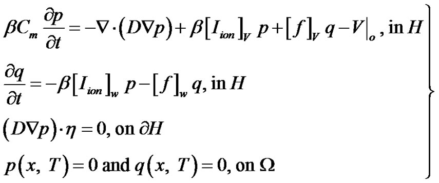 (15)
(15)
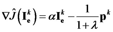
where Equation (14) is known as the state system while Equation (15) is known as the adjoint system. Also, from Equation (11), we can define the reduced gradient as follows
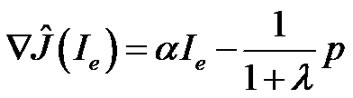 (16)
(16)
In order to compute the reduced gradient, we require solving the state system in Equation (14) forward in time, and then the adjoint system in Equation (15) backward in time.
Recall that the monodomain model consists of a parabolic PDE coupled to a system of nonlinear ODEs. Thus, the operator splitting technique [20] is applied to Equations (14) and (15) for decomposing the systems into sub-systems that are much easier to solve numerically. Consequently, the state system becomes
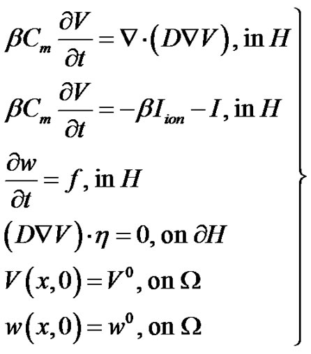 (17)
(17)
and the adjoint system becomes
 (18)
(18)
For the discretization procedure, the linear PDEs in Equations (17) and (18) are discretized with Galerkin finite element method in space and Crank-Nicolson method in time while the nonlinear ODEs in Equations (17) and (18) are discretized with forward Euler method in time. Thus, the discretized state system is given as
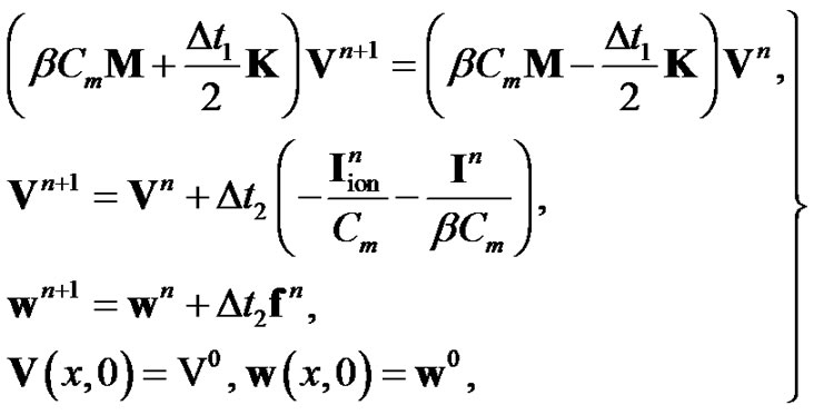 (19)
(19)
On the other hand,the discretized adjoint system is given as
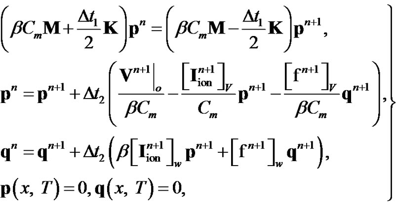 (20)
(20)
where  is the mass matrix,
  is the stiffness matrix,
  and
and  are the local time-steps. Once the state and adjoint systems have been discretized as shown in Equations (19) and (20), the optimization algorithms can be applied for solving the discretized optimal control problem.
4. Optimization Procedure
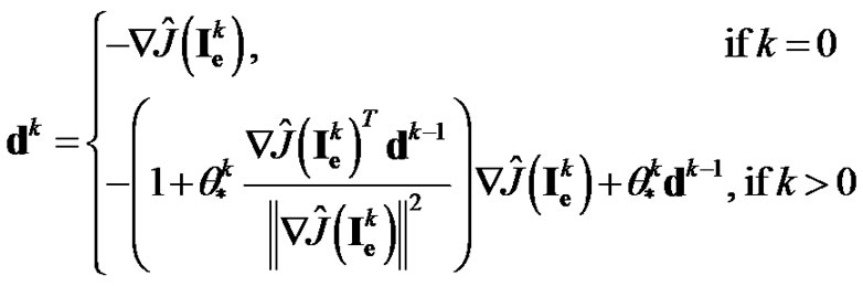
To solve the discretized optimal control problem of monodomain model, the modified Fletcher-Reeves (MFR) method [16] and modified Dai-Yuan (MDY) method [17] are used. Starting from an initial guess , the control variable is updated using the following recurrence
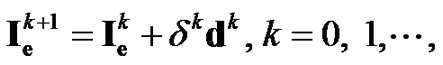 (21)
(21)
where  is the step-length and
  is the search direction defined by
 (22)
(22)
where  stands for the Euclidean norm of vectors and
  is the conjugate gradient update parameter. The conjugate gradient update parameters for the MFR and MDY methods are given as
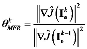 (23)
(23)
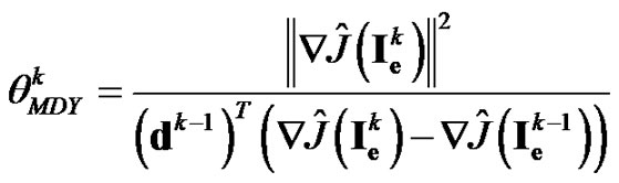 (24)
(24)
Recall that the FR and DY methods are descent methods with their descent properties depend on the line search, e.g. the Wolfe line search. On the other hand, the search directions for the MFR and MDY methods satisfy
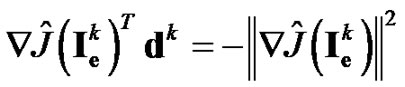 (25)
(25)
which is independent of any line search used. As a result, the MFR and MDY methods possess an advantageover the FR and DY methods since the Armijo line search can be used. Unlike the Wolfe line search, the Armijo line search only required us to solve the discretized state system in Equation (19). Consequently, the computational demand for solving the optimal control problem of monodomain model is reduced. Given an initial step-length , the Armijo line search choose
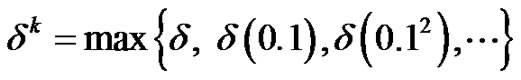
such that
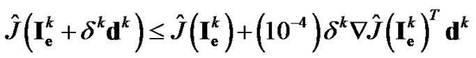 (26)
(26)
For the stopping criteria, we consider the following
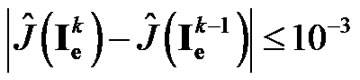 (27)
(27)
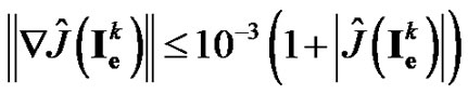 (28)
(28)
The optimization algorithm for solving the discretized optimal control problem is therefore given as follows.
Optimization Algorithm
Step 0. Provide an initial guess  and set
 .
.
Step 1. Solve the discretized state system in Equation (19).
Step 2. Evaluate the reduced cost functional .
.
Step 3. Use the result obtained in Step 1 to solve the discretized adjoint system in Equation (20).
Step 4. Update the reduced gradient
Step 5. For , check the stopping criteria in Equations (27) and (28). If one of them is met, then stop.
Step 6. Compute  using Equations (23) and (24).
Step 7. Compute  using Equation (22).
Step 8. Compute step-length  that satisfies condition in Equation (26).
Step 9. Update  using Equation (21). Set k = k+ 1 and go to Step 1.
5. Numerical Experiments
In this paper, the numerical experiments are carried out on a computational domain 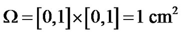 with final simulation time
 . Figure 1 illustrates the positions of the sub-domains in the computational domain
 . As shown in the figure,
  and
and  are the control domains,
  and
and  are the neighborhoods of the control domains,
  is the observation domain and
  is the excitation domain.
The parameters that are used in our numerical experiments are listed in Table 1, with some of them adopted from [21]. Furthermore, the initial values for V,  and
and  are given as
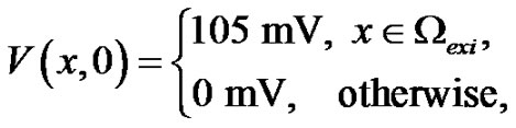 (29)
(29)
 (30)
(30)
 (31)
(31)
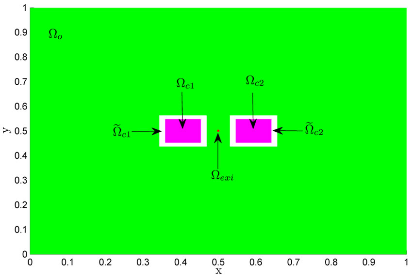
Figure 1. Computational domain  and its sub-domains.
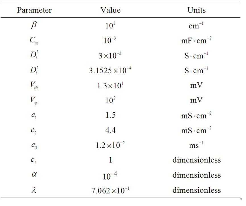
Table 1. Parameters used in numerical experiments.
Now, we present the experiment results for the optimal control problem of monodomain model using the MFR and MDY methods. The minimum values of the reduced cost functional  along the optimization process are depicted in Figure 2. Note that the logarithmic scale is used in Figure 2 for clear presentation on how the minimum values of the reduced cost functional are decreased during the optimization process.
As shown in Figure 2, the MDY method failed to converge to the optimal solution and stopped at iteration 14th. This result indicates that the global convergence of the MDY method is not guaranteed if the Armijo line search is used.
On the other hand, the MFR method successfully located the optimal solution by taking 618 iterations. This result shows that the MFR method is very efficient in real computations even if the Armijo line search is adopted. By comparing the results obtained by these two methods, we conclude that the MFR method outperforms the MDY method if the Armijo line search is considered.
The norm of the reduced gradient for the MFR and MDY methods are illustrated in Figure 3. As shown in the figure, the gradient for the MDY method keeps increasing from the beginning of the optimization process and finally stopped at iteration 14th. In contrast, the gradient for the MFR method starts decreasing from the beginning and finally approaches zero at the end of optimization iteration.
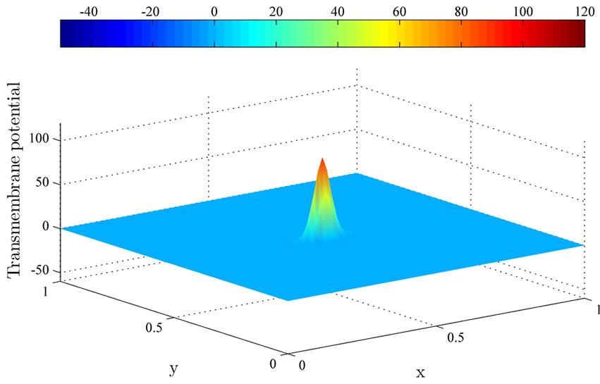
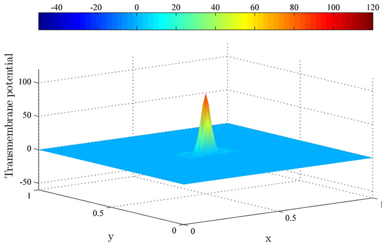
Figure 4 illustrates the uncontrolled solution at times 0.2 ms, 1 ms and 2 ms. The uncontrolled solution is obtained where no current is applied to the computational domain. Observe that the uncontrolled wavefront spreads
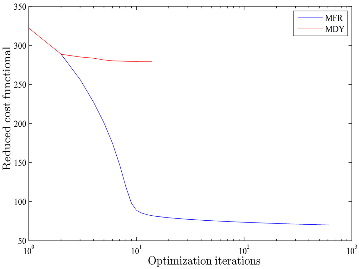
Figure 2. Minimum values of reduced cost functional  for 2 ms simulation time.

Figure 3. Norm of reduced gradient  for 2 ms simulation time.
 (a)
(a)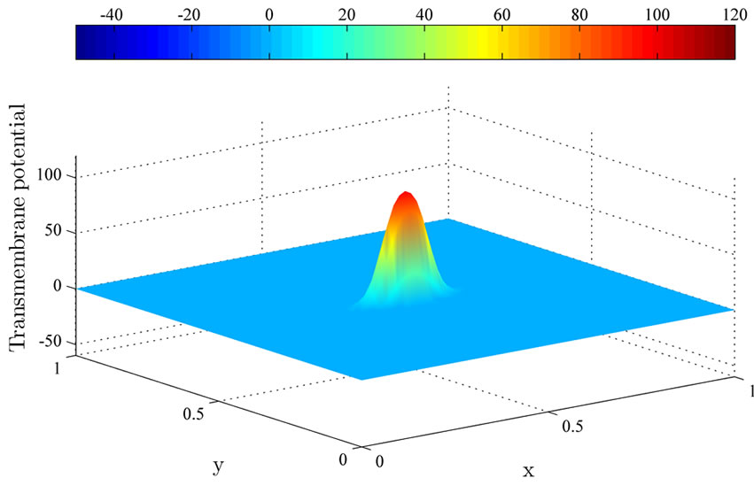 (b)
(b)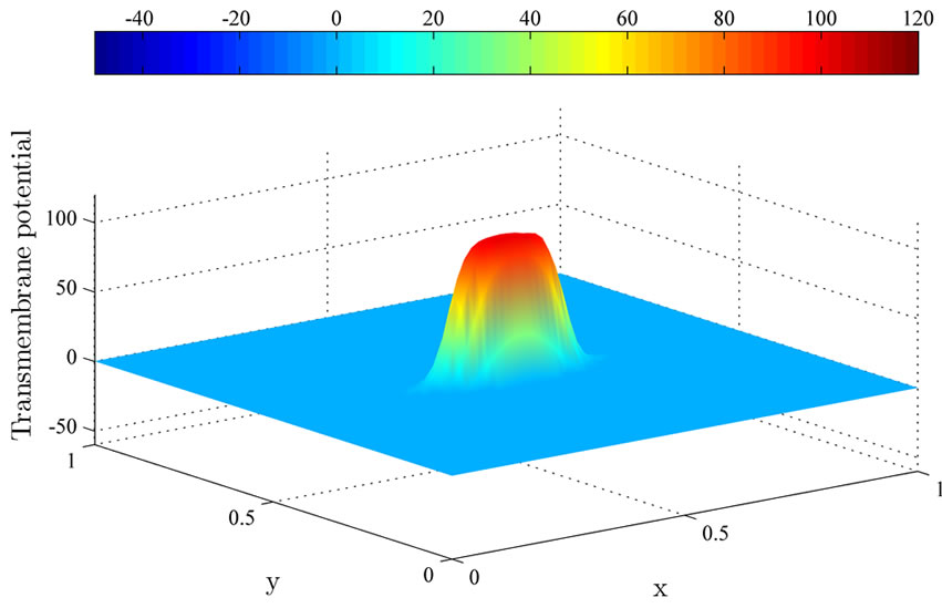 (c)
(c)
Figure 4. The uncontrolled solutions  at (a) 0.2 ms; (b) 1 ms; and (c) 2 ms.
from the excitation domain to the computational domain during the time interval from 0 ms to 2 ms. This implies that the excitation wavefront will continue to spread to the whole computational domain if no current is applied.
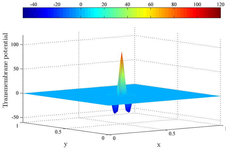
Figure 5 shows the controlled solutions at times 0.2 ms, 1 ms and 2 ms using the MFR method. As shown in the figure, the excitation wavefront is successfully dampened out by the optimal applied current . Moreover, the excitation wavefront is almost completely dampened out at time 1 ms.
 (a)
(a)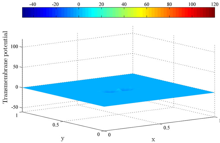 (b)
(b)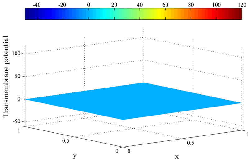 (c)
(c)
Figure 5. The controlled solutions  at (a) 0.2 ms; (b) 1 ms; and (c) 2 ms using the MFR method.
 (a)
(a)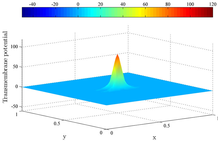 (b)
(b)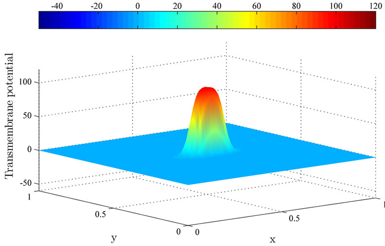 (c)
(c)
Figure 6. The controlled solutions  at (a) 0.2 ms; (b) 1 ms; and (c) 2 ms using the MDY method.
Next, the controlled solutions at times 0.2 ms, 1 ms and 2 ms using the MDY method are shown in Figure 6. Observe that the excitation wavefront is unable to be dampened out by the applied current, and the excitation wavefront continue to spread to the computational domain. This phenomenon happens because the MDY method failed to converge to the optimal solution  during the optimization process.
6. Conclusion
In this paper, we have presented the numerical experiment results for the optimal control problem of monodomain model using the modified Fletcher-Reeves method and modified Dai-Yuan method. Our experiment results show that the excitation wavefront is successfully dampened out by the optimal applied current when the modified Fletcher-Reeves method is used. However, when the modified Dai-Yuan method is employed, the excitation wavefront is not dampened out but continue to spread to the computational domain. We therefore conclude that the modified Fletcher-Reeves method outperforms the modified Dai-Yuan method when Armijo line search is used, and is suitable for solving the optimal control problem of monodomain model.
7. Acknowledgements
The work is financed by Zamalah Scholarship provided by Universiti Teknologi Malaysia and the Ministry of Higher Education of Malaysia.
REFERENCES
- Z. J. Zheng, J. B. Croft, W. H. Giles and G. A. Mensah, “Sudden Cardiac Death in the United States, 1989 to 1998,” Circulation, Vol. 104, 2001, pp. 2158-2163. doi:10.1161/hc4301.098254
- E. H. M. Ong, “Proposal for Establishment of a National Sudden Cardiac Arrest Registry,” Singapore Medical Journal, Vol. 52, No. 8, 2011, pp. 631-633.
- S. Zhang, “Sudden Cardiac Death in China,” Pacing and Clinical Electrophysiology, Vol. 32, No. 9, 2009, pp. 1159-1162.doi:10.1111/j.1540-8159.2009.02458.x
- C. Nagaiah, K. Kunisch and G. Plank, “Numerical Solution for Optimal Control of the Reaction-Diffusion Equations in Cardiac Electrophysiology,” Computational Optimization and Applications, Vol. 49, No. 1, 2011, pp. 149-178. doi:10.1007/s10589-009-9280-3
- S. M. Shuaiby, M. A. Hassan and M. El-Melegy, “Modeling and Simulation of the Action Potential in Human Cardiac Tissues Using Finite Element Method,” Journal of Communications and Computer Engineering, Vol. 2, No. 3, 2012, pp. 21-27.
- Y. Belhamadia, A. Fortin and Y. Bourgault, “Towards Accurate Numerical Method for Monodomain Models Using a Realistic Heart Geometry,” Mathematical Biosciences, Vol. 220, No. 2, 2009, pp. 89-101. doi:10.1016/j.mbs.2009.05.003
- C. Nagaiah and K. Kunisch, “Higher Order Optimization and Adaptive Numerical Solution for Optimal Control of Monodomain Equations in Cardiac Electrophysiology,” Applied Numerical Mathematics, Vol. 61, 2011, pp. 53- 65. doi:10.1016/j.apnum.2010.08.004
- E. Polak and G. Ribière, “Note Sur la Convergence de Méthodes de Directions Conjuguées,” Revue Francaise d’Informatique et de Recherche Opérationnelle, Vol. 16, 1969, pp. 35-43.
- B. T. Polyak, “The Conjugate Gradient Method in Extreme Problems,” USSR Computational Mathematics and Mathematical Physics, Vol. 9, 1969, pp. 94-112.doi:10.1016/0041-5553(69)90035-4
- W. W. Hager and H. Zhang, “A New Conjugate Gradient Method with Guaranteed Descent and an Efficient Line Search,” SIAM Journal on Optimization, Vol. 16, 2005, pp. 170-192. doi:10.1137/030601880
- Y. H. Dai and Y. Yuan, “A Nonlinear Conjugate Gradient Method with a Strong Global Convergence Property,” SIAM Journal on Optimization, Vol. 10, No. 1, 1999, pp. 177-182. doi:10.1137/S1052623497318992
- K. W. Ng and A. Rohanin, “Numerical Solution for PDEConstrained Optimization Problem in Cardiac Electrophysiology,” International Journal of Computer Applications, Vol. 44, No. 12, 2012, pp. 11-15.
- L. Zhang, “Two Modified Dai-Yuan Nonlinear Conjugate Gradient Methods,” Numerical Algorithms, Vol. 50, 2009, pp. 1-16. doi:10.1007/s11075-008-9213-8
- M. R. Hestenes and E. L. Stiefel, “Methods of Conjugate Gradients for Solving Linear Systems,” Journal of Research of the National Bureau of Standards, Vol. 49, No. 6, 1952, pp. 409-436.
- B. Ainseba, M. Bendahmane and R. Ruiz-Baier, “Analysis of an Optimal Control Problem for the Tridomain Model in Cardiac Electrophysiology,” Journal of Mathematical Analysis and Applications, Vol. 388, No. 1, 2012, pp. 231-247.doi:10.1016/j.jmaa.2011.11.069
- L. Zhang, W. J. Zhou and D. H. Li, “Global Convergence of a Modified Fletcher-Reeves Conjugate Gradient Method with Armijo-Type Line Search,” Numerische Mathematik, Vol. 104, 2006, pp. 561-572. doi:10.1007/s00211-006-0028-z
- L. Zhang, “Nonlinear Conjugate Gradient Methods for Optimization Problems,” Ph.D. Thesis, Hunan University, Changsha, 2006.
- J. M. Rogers and A. D. McCulloch, “A CollocationGalerkin Finite Element Model of Cardiac Action Potential Propagation,” IEEE Transactions on Biomedical Engineering, Vol. 41, No. 8, 1994, pp. 743-757. doi:10.1109/10.310090
- K. Kunisch and M. Wagner, “Optimal Control of the Bidomain System (I): The Monodomain Approximation with the Rogers-McCulloch Model,” Nonlinear Analysis: Real World Applications, Vol. 13, No. 4, 2012, pp. 1525- 1550. doi:10.1016/j.nonrwa.2011.11.003
- Z. Qu and A. Garfinkel, “An Advanced Algorithm for Solving Partial Differential Equation in Cardiac Conduction,” IEEE Transactions on Biomedical Engineering, Vol. 46, No. 9, 1999, pp.1166-1168. doi:10.1109/10.784149
- P. C. Franzone, P. Deuflhard, B. Ermann, J. Lang and L. F. Pavarino, “Adaptivity in Space and Time for ReactionDiffusion Systems in Electrocardiology,” SIAM Journal on Scientific Computing, Vol. 28, No. 3, 2006, pp. 942- 962.doi:10.1137/050634785