Applied Mathematics
Vol. 3 No. 6 (2012) , Article ID: 20085 , 8 pages DOI:10.4236/am.2012.36082
Basins of Attraction in the Copenhagen Problem Where the Primaries Are Magnetic Dipoles
1Department of Mechanics, Faculty of Applied Sciences, National Technical University of Athens, Athens, Greece
2Department of Mathematics, Faculty of Sciences, Aristotle University of Thessaloniki, Thessaloniki, Greece
Email: tkalvouridis@gmail.com, gousidou@math.auth.gr
Received March 14, 2012; revised April 11, 2012; accepted April 18, 2012
Keywords: Copenhagen Problem with Magnetic Dipoles; Equilibrium Locations; Basins of Attraction; Solution of Non-Linear Algebraic Systems; Newton and Quasi-Newton Methods; Comparison of Numerical Methods
ABSTRACT
We deal with the Copenhagen problem where the two big bodies of equal masses are also magnetic dipoles and we study some aspects of the dynamics of a charged particle which moves in the electromagnetic field produced by the primaries. We investigate the equilibrium positions of the particle and their parametric variations, as well as the basins of attraction for various numerical methods and various values of the parameter λ.
1. Introduction
The Copenhagen problem is a particular case of the famous restricted three-body problem where the two big spherical and homogeneous primaries have equal masses and rotate with constant angular velocity in circular orbits around their centre of mass, while a small massless particle moves under the resultant Newtonian action of the two primaries. The problem was exhaustively studied by Stromgren and his collaborators in the decade of 1920’s and has been revisited during the last ten years after the discovery of many exosolar planetary systems. A large part of these systems that have been identified since 1990, are two-body systems where the two primaries have almost equal masses. In this work we deal with a very interesting version of the Copenhagen problem in which we consider that the two big primaries are also magnetic dipoles and that the particle is a small charge which moves in the electromagnetic field produced by the two rotating dipoles. This new consideration besides the application to the aforementioned dynamical systems could also be applied to magnetic binary stars, the existence of which has been already confirmed. The dynamics of a charged particle in a magnetic binary system has been studied in the past ([1,2]). The material of this work is organized in four sections. In the first section we extract the equations of motion of the charged particle, in the second section we study the equilibrium positions, their stability and their parametric variation, in the third section we investigate the basins of attraction of these equilibria by applying two well known numerical methods, the Newton’s method and an improved Modified Broyden’s one. Finally, in the last section, we discuss the obtained results and we expose some of the major conclusions concerning our investigation.
2. The Problem
We consider a synodic coordinate system Oxyz centered at the mass centre O of the system, where the plane Oxy is the plane of the primaries’ motion, and the x-axis is the axis of syzygies of the primaries which create dipoletype magnetic fields. We assume that the axes of the magnetic moments are perpendicular to the Oxy plane and that the primaries rotate about their centre of mass in circular orbits with constant angular velocity ω (Figure 1). That is
 , i = 1, 2.
The magnetic inductions of the dipoles are,
 , i = 1, 2 where
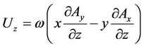
  are the vector potentials. From Faraday’s law we obtain
 , i = 1, 2.
A small particle of charge q and mass m is acted upon by a Lorentz’s force created by the two rotating primaries P1 and P2
 ,
,
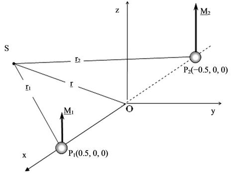
Figure 1. The configuration of the primaries-magnetic dipoles and the small body S.
where
 ,
, .
.
Under these assumptions, the normalized differential equations that describe the planar motion of S in the synodic coordinate system Oxyz, are,
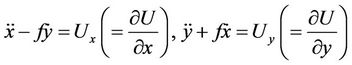 (1)
(1)
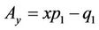
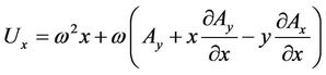
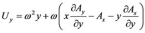
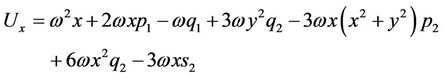
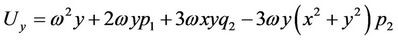
where
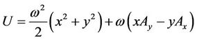
is the potential function, Ax, Ay are the x and y-components of the vector potential of the resultant electromagnetic field expressed in the synodic system, with
 ,
,  ,
,
 ,
, 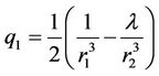
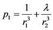
where r1 and r2 are the distances of the particle from the primaries,
 ,
,
 ,
,
 ,
,  ,
, 
or analytically,
and
with
 ,
,  ,
, 
The dynamical system is characterized by the parameter  which is the ratio of the two magnetic moments. Since parameter λ connects the magnitudes of these moments, its role in the formation of the resultant electromagnetic field is very important. From Equation (1) we obtain a Jacobian-type integral of motion which has the form
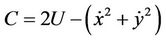 (2)
(2)
where C is a constant that is called the Jacobian constant or energy constant.
3. Equilibrium Locations and Their Parametric Variation
As it is known, in an equilibrium position on the plane of the primaries’ revolution the following conditions hold,
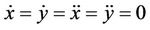 (3)
(3)
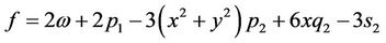
Therefore, the coordinates of these positions are the solutions of the system of non-linear algebraic equations,
 (4)
(4)
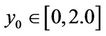
We have found that for our case where the magnetic moments are perpendicular on the plane of the primaries’ revolution, all the equilibrium positions of the particle are located on this plane. Some of these points are dynamically equivalent, which means that are characterized by the same Jacobian constant C and by the same state of stability. Τhe total number of the existing equilibrium locations depends on the value of parameter λ. More precisely:
• When  there are three collinear equilibrium positions (L1, L2, L3).
• When 2.6 ≤ λ ≤ 10.8, there are three collinear positions (L1, L2, L3) and four triangular positions that form two pairs (L4, L5) and (L6, L7). The points of each pair are symmetric with respect of the x-axis and are dynamically equivalent since they are characterized by the same Jacobian constant C and the same state of stability.
• When λ > 10.8 there are three collinear points (L1, L2, L3) and one pair of dynamically equivalent triangular points (L4, L5).
Figure 2 shows the distribution of these equilibria on the Oxy plane for various λ.
4. Methods and Algorithms for Finding the Basins of Attraction
4.1. Basins of Attraction
As we have mentioned before, in order to locate the equilibrium positions of the particle, we have to solve numerically the non-linear algebraic system (4). This is achieved by applying an iterative scheme, provided that an initial approximation is given. This starting value represents a point on plane (x, y). The iterator stops when some predetermined accuracy is reached for an equilibrium point which can be considered as an “attractor” of the method. We call the set of the initial points that lead to the discrete equilibrium points or the dynamically equivalent points, “basins of attraction” (or “basins of convergence”, or “attracting domains”). These regions have been studied in the past in some problems of Celestial Dynamics, such as the restricted three-body problem [3], the ring problem of (N + 1)-bodies [4-8], and the Hill’s problem with radiation and oblateness [9]. The technique to find these regions is based on a double scanning process of the Oxy plane. Here, we have considered the intervals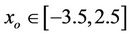 ,
,  for the vertical and the horizontal scanning respectively and a step equal to 0.005. We have created in this way a dense grid, the nodes of which are the initial values of the algorithm in use. In all the considered cases we have used 10−8 as the accuracy criterion to terminate the iterative process. We have stored in separate files all the initial points that lead to dynamically equivalent equilibrium points. At the same time, for each initial point, we have recorded the number of the iterations required to find the equilibrium position with the aforementioned accuracy. Naturally, the number of the iterations required to locate an equilibrium position depends on the predetermined accuracy, while the number of the points that
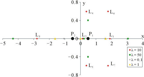
Figure 2. Distribution of the equilibrium positions for various values of λ.
constitute the set of the attracting domain of dynamically equivalent set of equilibrium positions depends on the step-size of the scanning process, and the method used. At this point we notice that many numerical methods solving systems of nonlinear algebraic equations have been proposed and described in the past (see for example [10,11]). In what follows we briefly describe the two algorithms used, that is, the old classic Newton’s algorithm and a modified version of Broyden’s iteration scheme.
4.2. The Numerical Methods Used
4.2.1. Newton’s Algorithm
For our particular problem this very popular and simple algorithm takes the form,
 (5)
(5)
 ,
,  are the values of x and y at the n-th approximation of the iteration process. Relations (5) can also be written in the form,
where  is the Jacobian matrix
 .
.
4.2.2. Modified Broyden’s Method
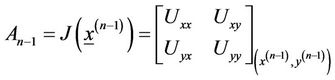
Broyden’s method is based on the secant’s one (it is a generalization of it) and belongs to a class of methods called quasi-Newton. We suppose that  is an initial solution
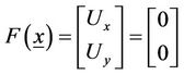
  of the non-linear system
and we compute the Jacobian matrix

and its inverse
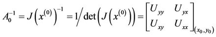
We calculate the next approximation in the same manner as in Newton’s method and then we determine
 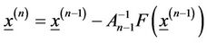 , for n = 2, 3, ∙∙∙solving the system
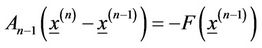 , at each step, until the criterion of convergence is satisfied. In this method
  has replaced the Jacobian matrix
  that appears in Newton-Raphson’s method.
This is the main difference between the two methods. Broyden’s method has convergence that is called “superlinear”; this implies that 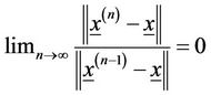 On the contrary, Newton’s method has a “quadratic” convergence. For our problem,
and
 (6)
(6)
for Broyden’s method, where  is given by the formula:
 (7)
(7)
where . This method has been applied by Gousidou and Kalvouridis [5-8].
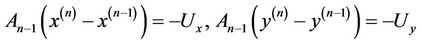
An improvement of Broyden’s method is based on the Sherman-Morrison’s matrix inversion formula. This formula computes the inverse matrix  directly from
 , eliminating in this way, the need for a matrix inversion in each iterative step. So, we have not to inverse the matrix
 , which appears in Newton’s method
 (8)
(8)
and not need to solve a system
with
 in each iteration, as it is needed in Broyden’s method. Its convergence is also “superlinear”, but with less number of operations than the original Broyden’s method, since the operations that are needed are those for the multiplication of a matrix by a vector, as it is resulted from the formula:
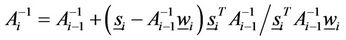 (9)
(9)
where

and
 , for
, for , (10)
(Faires and Burden [12]).
5. Discussion of the Results
5.1. General Remarks and Comments
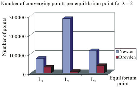
Newton-Raphson’s method gives a greater number of converging points per equilibrium point, in comparison to Broyden’s method which gives a few number of converging points. This is shown in the bar charts of Figure 3 for the three considered cases with λ = 2, 10 and 12.
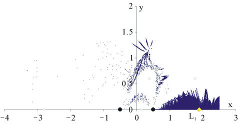
The general structure of the obtained basins of attracttions generally consists of some very dense parts that mainly evolve around the respective equilibrium point and of dispersed points that lie on the boundaries of the dense regions of this equilibrium or other ones. Figures 4-7 illustrate the results obtained from our investigation. The two methods provide results showing similarities and differences that mostly arise from the philosophy and the geometric origin of the individual method.
Fundamental similarities:
• In all diagrams, the shapes of the central parts of the corresponding attracting regions that evolve in the neighborhood of the dynamically equivalent equilibrium points are similar.
• The boundaries of these central parts are not clearly defined. They look as if they are being unraveled or unweaved. If one chooses launching points near these boundaries, very slight differences can give rise to very different outcomes.
Substantial differences:
• The central parts of the dense regions of NewtonRaphson’s method are “compact” and homogeneous, that is, all their points lead to the equilibrium positions of a particular set and therefore show the deterministic aspect of these areas for the particular numerical method. On the contrary, the corresponding regions obtained by means of modified Broyden’s method are less extended and less cohesive than the previous ones.
• The initial approximations of plane (x, y) which do not lead to a target in the Newton-Raphson method, are very few. On the contrary, in the modified Broyden’s method, a great number of non-convergent initial approximations exists. Most of them are located at a relatively great distance from the primaries and are distributed in some extended areas of the diagram.
Newton-Raphson’s method “strikes” the target very fast, after a very few iterations. On the contrary, Broyden’s method needs many more iterations to achieve
 (a)
(a)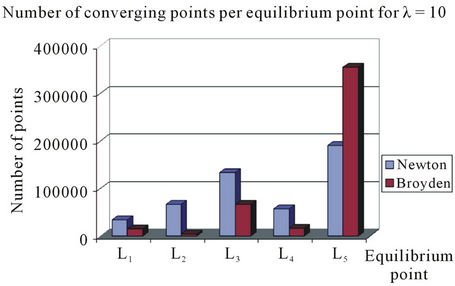 (b)
(b)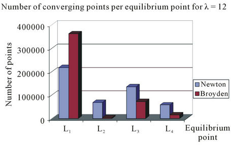 (c)
(c)
Figure 3. Bar charts showing the number of converging points per equilibrium point or equilibrium set in each numerical method used. (a) λ = 2; (b) λ = 10; (c) λ = 12.
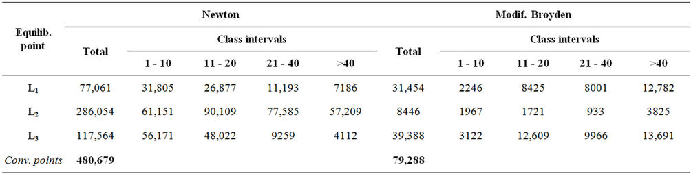
convergence. This is depicted in the bar charts of Figure 3 as well as in the Table 1 where we give the results obtained for the three considered cases with λ = 2, 10 and 12.
5.2. Sub-Regions of High or Low Speed of Convergence
We have extended our investigation by studying the way with which the attracting domain of an equilibrium point or set is resolved into smaller regions, according to the number of the iterations needed to reach the equilibrium
 (a)
(a)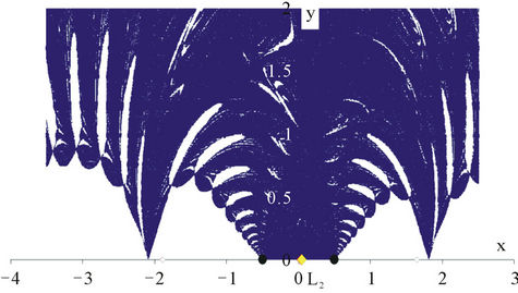 (b)
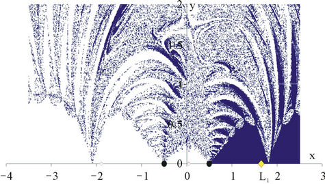
(b)
Figure 4. λ = 2. Newton’s method. Basins of attraction of the equilibrium points: (a) L1; (b) L2.
 (a)
(a)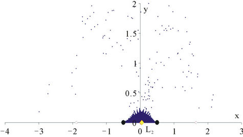 (b)
(b)
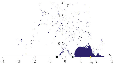
Figure 5. λ = 2. Modified Broyden’s method. Basins of attraction of the equilibrium points: (a) L1; (b) L2.
 (a)
(a)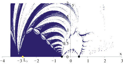 (b)
(b)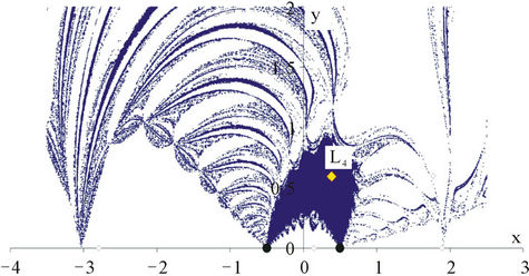 (c)
(c)
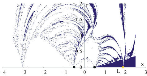
Figure 6. λ = 10. Newton’s method. Basins of attraction of the equilibrium points: (a) L1; (b) L3; (c) L4.
positions of this particular set. As we have already stressed in the previous section, the number of the required iterations in order to achieve the location of an equilibrium position depends on the predetermined accuracy. In order to provide clear and instructive pictures, we have classified the points of the attracting regions of each equilibrium set and for both methods used in this work, in four class intervals 1 - 10 (very fast convergence), 11 - 20 (fast convergence), 21 - 40 (moderate convergence) and >40 (slow or very slow convergence) for the number of iterations and accuracy of 10−8.
The general observations that concern all sets of points and both methods can be summarized as follows:
• The subset of the “launching” points of (x, y) plane corresponding to the class interval 1 - 10 iterations for any equilibrium position of any equilibrium set, consists of a small region which occupies the central part
 (a)
(a)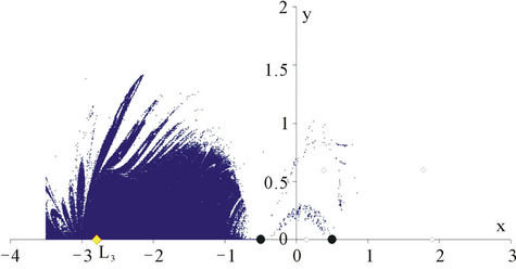 (b)
(b) (c)
(c)
Figure 7. λ = 10. Modified Broyden’s method. Basins of attraction of the equilibrium points: (a) L1; (b) L3; (c) L4.
of the attracting domain around each equilibrium position of this particular set and of some dispersed points, which appear near these areas or between the dense regions of other equilibria or sets. Regarding Modified Broyden’s method this class appears as a sparse cluster of points that are scattered among the points of the second class.
• The subset of the points corresponding to the class interval 11 - 20 iterations of each set consists of regions or points which complement the central regions of the first class interval and of a large number of isolated points in the attracting area of this particular equilibrium point or set. These points are spread in a widely extended area on (x, y) plane.
• The points corresponding to the class interval 21 - 40 iterations of each set evolve in a similar way as in the previous class.
 (a)
(a)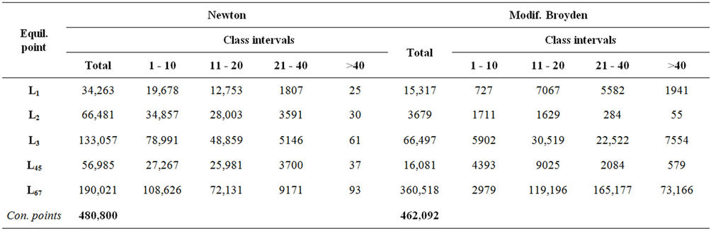 (b)
(b)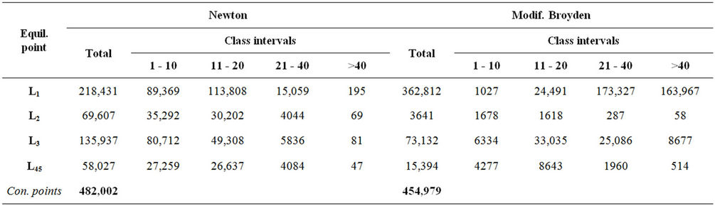 (c)
(c)
Table 1. Number of converging points per class interval.(a) λ = 2; (b) λ = 10; (c) λ = 12.
• Regarding class interval > 40 iterations, it merely consists of dispersed points lying either on the boundaries of the dense regions of the previously mentioned class interval, or between the dense regions of the other equilibrium points or sets. Naturally, a decreasing density is observed as the number of iterations increases.
6. Conclusion
We have investigated the attracting areas for the equilibria of a charged particle in a magnetic binary system using both Newton’s and Modified Broyden’s methods. In this system the number of equilibria depends on the values of parameter λ and the attracting domain of each dynamically equivalent set of equilibria consists of a dense sub-domain in the close neighbourhood of each equilibrium point of this set and of dispersed points distributed at the boundaries of the former domain of the same or other equilibrium sets. These boundaries are not clear and in some cases present a fractal structure. The application of the two methods reveals similarities and differences that exist between them. The dense part of an attracting region calculated with Newton’s method is more “compact” than the respective one calculated with Modified Broyden’s method. Another difference concerns the dispersed points. When these points are calculated with Newton’s method they are distributed in an extended area of the diagram and mainly on the boundaries of the “compact” regions. In Modified Broyden’s method these points are very few and in many cases form small point clusters beyond or near the central domain. We also observe that Newton’s method “strikes” the final target very fast. For the vast majority of the initial approximations, the method needs only 1 - 10 iterations. On the contrary, Modified Broyden’s method needs often many more iterations to achieve convergence. Figures 3-7 and Table 1 justify our remarks. The presented material confirms that Newton’s method is more efficient than Modified Broyden’s one (for this type problem) as regards all the indices examined, such as the speed of convergence and the total number of launching points of the xy-plane that lead to the desired final destination.
REFERENCES
- T. J. Kalvouridis and A. G. Mavraganis, “Symmetric Motions in the Equatorial Magnetic-Binary Problem,” Celestial Mechanics, Vol. 40, No. 2, 1987, pp. 177-196. doi:10.1007/BF01230259
- T. J. Kalvouridis, “Three-Dimensional Equilibria and Their Stability in the Magnetic-Binary Problem,” Astrophysics and Space Science, Vol. 159, No. 1, 1989, pp. 91-97. doi:10.1007/BF00640490
- M. Croustalloudi and T. J. Kalvouridis, “Structure and Parametric Evolution of the Basins of Attraction in the Restricted Three-Body Problem,” Proceedings of the 7th National Congress on Mechanics, Chania Crete, Vol. 2, 24-26 June 2004, pp. 144-150.
- M. Croustalloudi and T. J. Kalvouridis, “Attracting Domains in Ring-Type N-Body Formations,” Planetary and Space Science, Vol. 55, No. 1, 2006, pp. 53-69. doi:10.1016/j.pss.2006.04.008
- M. Goussidou-Koutita and T. J. Kalvouridis, “A Comparative Study of the Attracting Regions in the Ring Problem of (N + 1) Bodies,” International Conference of Computational Methods in Science and Engineering, Chania Crete, 8 April 2006.
- M. Gousidou-Koutita and T. J. Kalvouridis, “Application of Newton and Broyden Methods for the Investigation of the Attracting Regions in the Ring Problem of (N + 1) Bodies: A Comparative Study,” Abstracts of the Conference Gene around the World, Tripolis, 29 February-1 March 2008, p. 2.
- M. Gousidou-Koutita and T. J. Kalvouridis, “Numerical Study of the Attracting Domains in a Non-Linear Problem of Celestial Mechanics,” Recent Approaches to Numerical Analysis: Theory, Methods and Applications, Conference in Numerical Analysis, Kalamata, 1-5 September 1998, pp. 84-87.
- M. Gousidou-Koutita and T. J. Kalvouridis, “On the Efficiency of Newton and Broyden Numerical Methods in the Investigation of the Regular Polygon Problem of (N + 1) Bodies,” Applied Mathematics and Computing, Vol. 212, No. 1, 2009, pp. 100-112. doi:10.1016/j.amc.2009.02.015
- Ch. Douskos, “Collinear Equilibrium Points of Hill’s Problem with Radiation and Oblateness and Their Fractal Basins of Attraction,” Astrophysics and Space Science, Vol. 326, No. 2, 2010, pp. 263-271. doi:10.1007/s10509-009-0213-5
- M. N. Vrahatis and K. I. Iordanidis, “A Rapid Generalized Method of Bisection for Solving Systems of Non- Linear Equations,” Numerische Mathematik, Vol. 49, No. 2-3, 1986, pp. 123-138. doi:10.1007/BF01389620
- V. Drakopoulos and A. Bohm, “Basins of Attraction and Julia Sets of Shröder Iteration Functions,” In: A. Bountis and S. Pnevmatikos, Eds., Proceedings of the 7th and 8th Summer Schools on Non-Linear Dynamical Systems, Vol. 4, 1998, pp. 157-163.
- D. J. Faires and R. L. Burden, “Numerical Methods,” PWS-KENT Publ. Co., Boston, 1993.