Applied Mathematics
Vol. 3 No. 1 (2012) , Article ID: 16767 , 6 pages DOI:10.4236/am.2012.31007
Some Kinds of Sheaf Control Problems for Control Systems
Faculty of Mathematics and Computer Science, Vietnam National University, Ho Chi Minh City, Vietnam
Email: *ndphu_dhtn@yahoo.com.vn
Received November 8, 2011; revised December 20, 2011; accepted December 27, 2011
Keywords: Control Systems; Sheaf Solutions; Control Theory
ABSTRACT
Recently, the field of differential equations has been studying in a very abstract method. Instead of considering the behaviour of one solution of a differential equation, one studies its sheaf-solutions in many kinds of properties, for example, the problems of existence, comparison, … of sheaf solutions. In this paper we study some of the problems of controllability for sheaf solutions of control systems.
1. Introduction
In [1-4] the authors have investigated sheaf solutions of control differential equations in the fields: comparison of sheaf solutions in the cases’ two admissible controls  and
and , and some initial conditions
 ,
,  , where the Hausdorff distance between the sets of initials
  and
and  is enough small.
The problems of sheaf controllability and sheaf optimization are still open. The present paper is organized as follows. In Section 2, we review some facts about sheaf solutions. In Section 3 we give many kinds of sheaf control problems, of sheaf controllability optimal problems.
2. Preliminaries
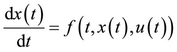
In n-dimension Euclidian space  usually we have considered the control systems (CS):
 (2.1)
(2.1)
where ,
, 
 . A solution to CS (2.1) is represented by:
 (2.2)
(2.2)
 ,
,  ,
,  is a collection of some given initials.
Definition 2.1. We say that a control  is admissible, if:
1)  satisfies (2.2) for all
 ;
;
2)  is bounded by norm
 .
.
That means the functions  are measurable (integrable) satisfiying almost everywhere on
  the relationships (2.1) and (2.2), then
  is called the trajectory of the CS (2.1) and
  is called the control. Therefore, we shall always understand a pair of functions
  interrelated by the relationship (2.1) and (2.2). It is clear that several controls
  can correspond to one
  trajectory and if CS (2.1) has a nonunique solution, then several trajectory
  can correspond to one control
 .
.
Definition 2.2. A state pair  of solutions of control systems (2.1) will be a controllable if after time
  we shall find a control
  such that:
 (2.3)
(2.3)
Definition 2.3. A control system (2.1) is said to be:
(GC) global controllable if every state pair of set solution .
.
(GA) global achievable if for every  we have a state pair of solutions
  that is GC.
(GAZ) global achievable to zero if for every  we have a state pair
  that will be controlable.
In [2] the authors have compared the sheaf solutions for set control differential equations (SCDEs).
In [4] the author has study the problems (GC), (GA) and (GAZ) for set control differential equations (SCDEs).
Definition 2.4. A sheaf solution (or sheaf trajectory)  is denoted by a number of solutions that make into sheaves (lung one on top of the other and often tied together) for all
 :
:
 (2.4)
(2.4)
Definition 2.5. A cut-set (a cross-area) of sheaf solution  at time
  is denoted by:
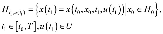 (2.5)
(2.5)
3. Main Results
Let’s consider again the control systems (CS):
 (3.1)
(3.1)
where ,
,  , Q is a compact set in
  and
and —admissible controls. Assume that for CS (3.1) there exists solution (2.2) and sheaf solution (2.4).
We will need the following hypotheses on the data of control problem for CS (3.1):
(Hf1): 
(Hf2): 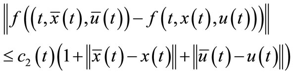
where .
.
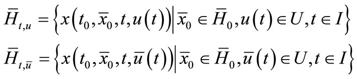
Assume that at all ,
,  for two admissible controls
  we have two forms of sheaf solutions:
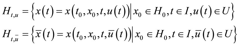 (3.2)
(3.2)
where —solution of CS (2.1) (see Figure 1).
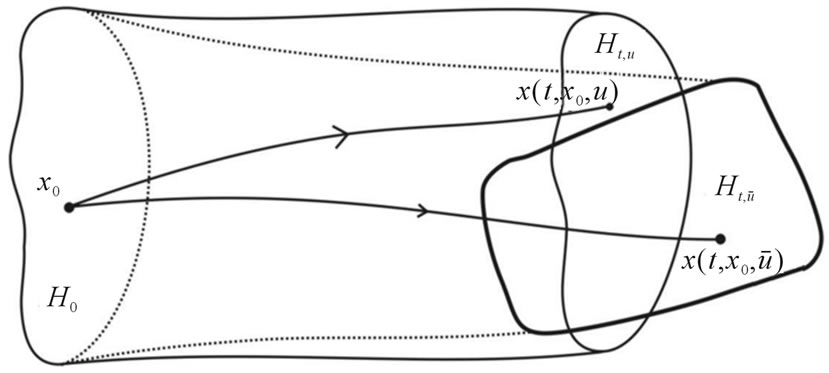
Figure 1. The sheaf solutions of CS (2.1) in two admissible controls.
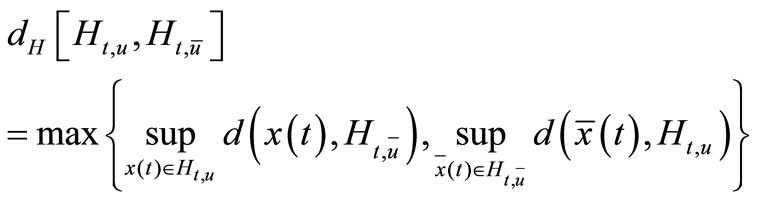
Definition 3.1. The Hausdorff distance between set  and
and  is denoted by:
Definition 3.2. The pair of the any sets  will be controllable if after time
  we shall find a control
  and one map
  such that:
 (3.3)
(3.3)
Theorem 3.1. Under Hypothes (Hf1), let  —is initial, any set
 . The pair of the sets
  will be controllable if:
1)  belongs to solutions of CS (3.1), and 2)
  is cut-set of sheaf solution to (3.1), that means
 .
.
Proof. If  belongs to solutions of CS(3.1) then it is
 .
.
For any  we have a pair
  that is controllable, because
 , where
  —cut-set of sheaf solutions with
As in results, we have one map moving  to
to  that means
 .
.
Definition 3.3. The control system (3.1) is said to be:
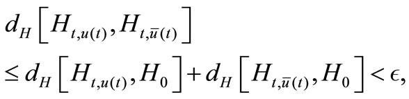
(SC1) sheaf controllable in type 1, if for all , there exists
  and admissible controls
  that satisfy
  then
then
 (3.4)
(3.4)
(SC2) sheaf controllable in type 2 for any admissible control , if for all
 , there exists
  such that the initials
 with
with  then
then
 (3.5)
(3.5)
(SC3) sheaf controllable in type 3, if for all , there exist
 ,
,  such that the initials
 with
with  and for any admissible controls
  that satisfy
  then
then
 (3.6)
(3.6)
Lemma 3.1. Under Hypothes (Hf1), for all , there exists
  if control system (3.1) with:
then two cut -sets of sheaf-solutions of CS (3.1) satisfy an estimate:
 (3.7)
(3.7)
Proof. Suppose that for CS (3.1) the right hand side  satisfies (Hf1) then there exists unique solution
  which satisfies (2.2).
If —sheaf solution of CS (3.1) then for admissible control
  we have the cut-sets at any times
 , that satisfy estimate (3.7):
 and
and .
.
We have

Theorem 3.2. Assume that, under Hypothes (Hf2), the admissible controls  that satisfy
  , then CS (3.1) is sheaf-controllable SC1.
Proof. Suppose that for CS (3.1) the right hand side  satisfies (Hf2) then there exists unique solution
  which satisfies (2.2).
If —sheaf solution of CS (3.1) then for admissible control
  we have the cut-sets at every times
 , that satisfy estimate (3.7):
  and
and .
.
We have
as results the CS (3.1) is sheaf-controllable SC1. 
Corollary 3.1. If CS (3.1) is SC1, the right hand side  satisfies condition of lemma 3.1 then for all
  there exists
  such that:
Proof. Because solution of CS (3.1) is equivalent: 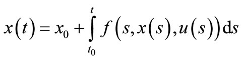 then
then

by lemma 3.1 we have:

Theorem 3.3. Under hypothes (Hf1), assume that the initials  for all
 , there exists
  such that:
  then for any admissible control
  we have:
that means CS (3.1) is sheaf controllable CS2.
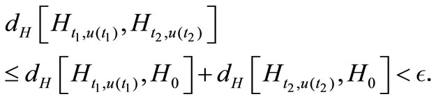
Proof. We have estimate
For all ,
,  such that
 and
and
 choosing
  then we have
 . As results imply that CS (3.1) is SC2.
Theorem 3.4. Under Hypothes (Hf2), assume that for all  and satisfy the followings:
1) 
2) then for any admissible controls
  we have:

that means CS (3.1) is sheaf controllable CS3.
Proof. Beside (2.4) for  and
and  we have:
and estimate  as following:
Choosing , we have:

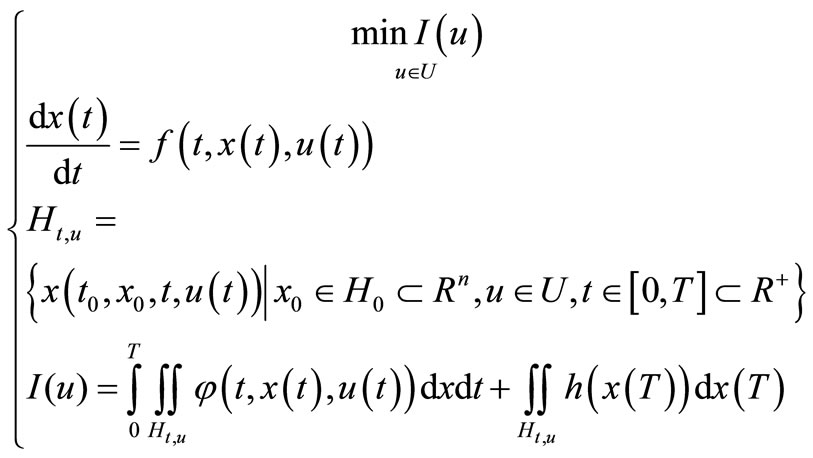
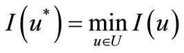
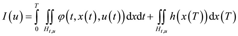
Definition 3.4. We say that for control system (3.1) are given OCP—the optimization control problem if it denotes:
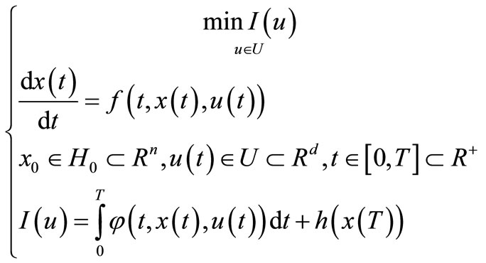 (3.8)
(3.8)
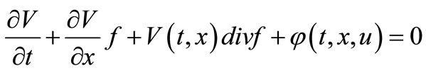
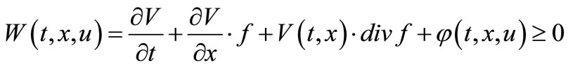
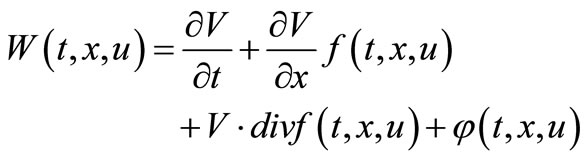
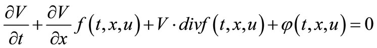
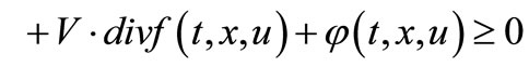
where , such that V(T,x) is solution to Hamillton Jacobi Bellman (HJB)—partial differential equation:
 (3.9)
(3.9)
We have to find the optimal control  for OCP (3.8).
Lemma 3.1. In optimization control problems (3.8) if  then
then 
Proof. Putting 
we have integral for all :
:
Because
impilies that

Theorem 3.5. Assume that OCP (3.8) has  and there exists feedback
 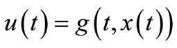 such that:
then exists optimal control  for OCP (3.8).
Proof. Assume that —one of solutions of control systems (3.1) such that
  there exists feedback
 :
:
By lemma 3.3 we have
such that —optimal control for OCP (3.8).
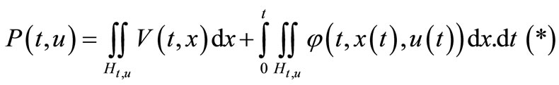
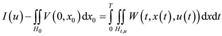
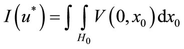
Definition 3.5. We say that for control system (3.1) are given SOCP—the sheaf-optimization control problem if it denotes:
 (3.10)
where —integral on
  and
and
 such that
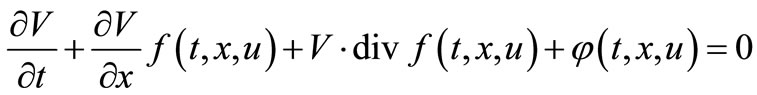
  is solution to (HJB)—partial differential equation:
 (3.11)
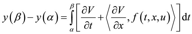
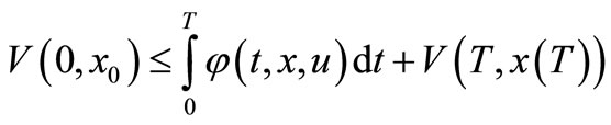
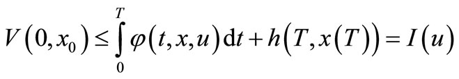
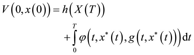
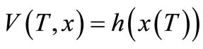
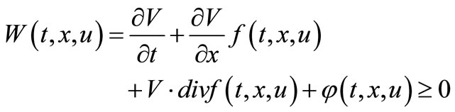
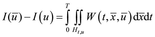
Lemma 3.2. Assume that V(t, x) is a solution of HJB partial differential equation (3.10) with the boundary conditions:

If function
and u(t) is admissible control then for optimization control problem SOCP (3.10) there exists estimate:

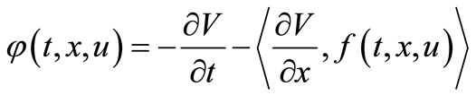
Proof. Putting
we have:
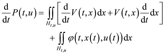
 where
where 
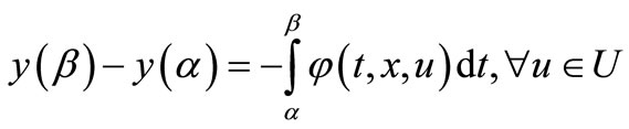
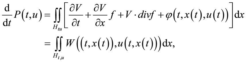
then
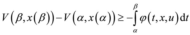
By (*) we have
and  then (**) impilies that

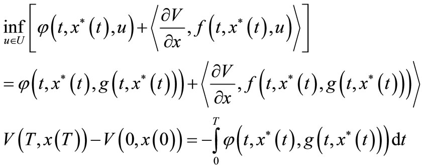
Theorem 3.6. (Necessary Conditions)
Assume that SOCP (3.10) has solution, that means there exists optimal control  such that
 and
and  is a solution of HJBpartial differential equation (3.11) then the necessary conditions for this SOCP (3.10) are:
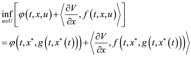
1) 
2) , where
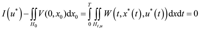
Proof. Suppose that a function SOCP (3.10) that means
 . Because V(t, x)-solution of HJBpartial differential equation (3.11):
with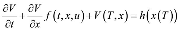 if function
  satisfies:
that integrable on sheaf solutions .
.
By lemma 3.2, if  is admissible control then for optimization control problem SOCP (3.10) there exists estimate:

Assume that for SOCP (3.10) has optimal control  then for all
 , we have
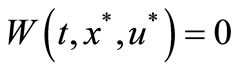

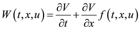
Theorem 3.7. (Sufficient Conditions)
Assume that  any admissible control for SOCP (3.10) and
  is a solution of HJB-partial differential Equation (3.11) then the sufficient conditions for this SOCP (3.10) are:
1) 
2) 
3) there exists  such that
Proof. There exists the other admissible control , such that for SOCP (3.10) we have
By condition (1) of theorem 3.6 we have a function

that integrable on sheaf solutions .
.
We find the function  from equation:
with condition .
.
By condition (2) of this theorem:
and implies that —optimal control for SOCP (3.10).
Example 3.1. When using missiles not for the purpose of shooting down aircraft noise bomb attack as B52 shot if only 01 or 02 rockets can not succeed. The rockets theit fire it will be the interference or escort aircraft will be explosive.
A problem arises: What to do in order to shoot down aircraft noise when operating in the sky. To solve this problem, we must fire simultaneously from SAM sites from 03 or more results. The rockets have to be controlled from headquarters and shot to pick the exact point-B52.
Mathematical model for problem shooting attack aircraft noise control system with (3.10), the test bundle (2.4) and optimization problem are (SOCP) in the above with n = 3 (see Figure 2).
4. Conclusions
The Sheaf Optimization problem for Control Systems
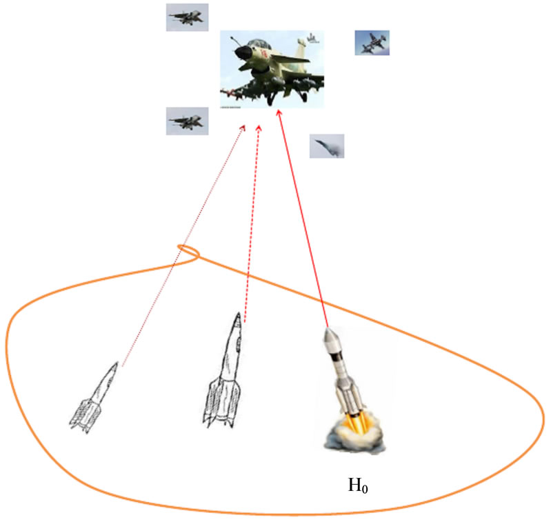
Figure 2. The sheaf of SAM shooting down aircraft noise bomb attack as B52.
(SOPCS) have a high practical significance, as the series of SAM to destroy B52 attack aircraft with fighter jamming, or laser beam to destroy targets, like the beams in materials research of Physical nuclear, etc, … This paper described some types of sheaf optimal problems. We can solve them by Pontryagin’s Principle, Lyapunov’s Energy Function or by the Hamilton’s Principle. In this paper we present the necessary and sufficient conditions for this problem by Hamilton’s Principle, namely by HJB equations.
In the near future, we will set the numerical calculations can be applied to a clearer and will study the different Optimization problems with some controls .
.
5. Acknowledgements
The authors gratefully acknowledge the referees for their careful reading and many valuable remarks which improved the presentation of the paper.
REFERENCES
- A. D. Ovsyannikov, “Mathematical methods in sheaf controls,” Leningrad University Pub., Saint Petersburg, 1980.
- N. D. Phu and T. T. Tung, “Some properties of sheafsolutions of sheaf fuzzy control Problems,” Electronic Journal of Differential Equations, Vol. 2006, No. 108, 2006, pp. 1-8.
- N. D. Phu and T. T. Tung, “Some results on sheaf solutions of sheaf set control differential equations,” Journal of Nonlinear Analysis: Theory, Methods & Applications, Vol. 67, No. 5, 2007, pp. 1309-1315. doi:10.1016/j.na.2006.07.018
- N. D. Phu, “On the Global Controllable for Set Control Differential Equations,” International Journal of Evolution Equations, Vol. 4, No. 3, 2009, pp. 281-292.
NOTES
*Corresponding author.