Wireless Engineering and Technology
Vol. 3 No. 4 (2012) , Article ID: 24195 , 4 pages DOI:10.4236/wet.2012.34033
Energy Detector with Baseband Sampling for Cognitive Radio: Real-Time Implementation
![]()
Electrical Engineering Department, College of Engineering, University of Baghdad, Baghdad, Iraq.
Email: mahmood.abdulsattar@googlemail.com, alsulaimawi@yahoo.com
Received June 14th, 2012; revised July 12th, 2012; accepted July 22nd, 2012
Keywords: Real-Time Implementation; Cognitive Radio (CR); Energy Detection
ABSTRACT
Cognitive radio (CR) is a technology that provides a promising new way to improve the efficiency of the use of the electromagnetic spectrum that available. Spectrum sensing helps in the detection of spectrum holes (unused channels of the band), and instantly move into vacant channels while avoiding occupied ones. An energy detector with baseband sampling for CR is presented with mathematical analyses for an additive white Gaussian noise (AWGN) channel. A brief overview of the energy detection based spectrum sensing for CR technology is introduced. Practical implementation issues on Texas Instruments TMS320C6713 floating point DSP board are presented. Novelties of this work came from a derivation of probability of detection and probability of false alarm for the baseband energy detector without including the sampling theorems and the associated approximation.
1. Introduction
The limited available spectrum and inefficiency in the use of the spectrum makes it necessary to establish the new communication model to benefit from the existing wireless spectrum professionally.
Mitola proposed a solution to the spectrum efficiency problem [1], where higher spectrum efficiency can be reached by dynamic spectrum access [2,3]. The concept of cognitive radio (CR) allows detecting the unused spectrum (spectrum holes) of the primary user (PU) in order for the secondary user (SU) to share the spectrum without harmful interference. The accuracy of detection is the most important factor that determines the performance of the CR. Since the concept of CR is still at the stage of being developed, there is no agreement on what kind of wireless technologies to employ for realizing it. Currently, there are three different techniques which are commonly used in signal processing techniques for spectrum sensing [4]: matched filter, cyclostationary feature detection and energy detection.
In [5], the matched filter also referred to as coherent detector, it can improve detection performance if the primary transmitted signal is deterministic and known a priori. This technique can be applied only when we choose to detect specific signals, and it is very accurate since it maximizes the SNR for the signal.
In [6,7], a signal is said to be cyclostationary if its mean and autocorrelation are a periodic function. Communication signals may have special statistical features. Feature detection denotes to extracting features from the received signal and performing the detection based on the extracted features. Cyclostationary feature detection can distinguish PU signal from noise, and used at very low signal to noise ratio (SNR) detection by using the information embedded in the PU signal that is not presented in the noise. The main drawback of this method is the complexity of calculation. Also, it must deal with all the frequencies in order to generate the spectral correlation function, which makes it a very large calculation. The benefit of feature detection compared to energy detection is that it typically allows differences among dissimilar signals or waveforms.
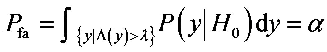
Energy detection (also denoted as noncoherent detection), is the signal detection mechanism using an energy detector (also known as radiometer) to specify the presence or absence of signal in the band. The most often used approaches in the energy detection are based on the Neyman-Pearson (NP) lemma. The NP detection criterion enlarges the probability of detection for a given probability of false alarm
 .
.
It is an essential and a common approach to spectrum sensing since it has moderate computational complexities, and can be implemented in both time domain and frequency domain [8,9]. In [10], to adjust the threshold of detection, energy detector requires knowledge of the power of noise in the band to be sensed. The signal is detected by comparing the output of energy detector with threshold which depends on the noise floor.
The TMS320C6713 kit was chosen as it provides a properly low cost access into the real-time implementation of energy detection algorithms. This DSP card has the following features: It evaluates 1350 million floating point operations per second (MIPS), a processor running at 225 MHz, programmed by C and assembly languages.
The paper is organized as follows: Section 2 describes detection techniques. Section 3 lists the main issues of previous works. Section 4 presents the baseband energy detector model. Section 5 drives probability equations for baseband energy detector over AWGN Channel. Section 6 describes how to generate noisy PU signal. Section 7 implemented using a DSP kit. Discussed in Section 8 presented. Finally, in Section 9 the conclusions are mentioned .
2. Detection Techniques
Fundamental to the theory of detecting the signal in noise is the theory of statistical decision, where the decision-making depends on the hypothesis testing. In binary hypothesis testing, the problem resides in defining a decision rule that indicates which of two hypotheses should be chosen: the null hypothesis ( ) or the alternative hypothesis (
 ). If the null and alternative hypotheses are defined in terms of signal(s), hypothesis
  (signal absent) and hypothesis
  (signal present).
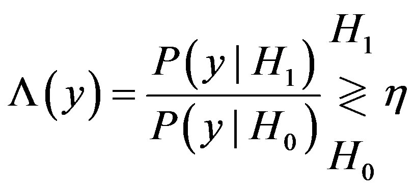
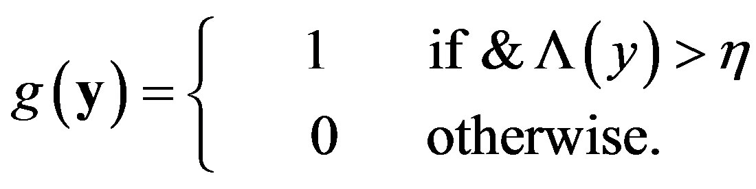
In [11], the decision rule can be represented as
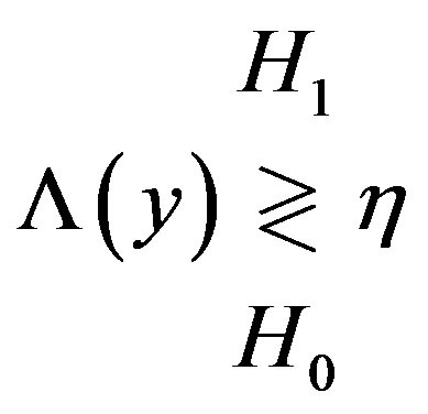 (1)
(1)
where  is the threshold and
  is a function that depends on the measurements. If it exceeds the threshold, then
  is selected; otherwise,
  is decided. The aim of the detection theory is, hence, to design the most effective detector by definition
 and
and . Let
. Let  be the observation vector and
  denote the joint probability density function (PDF) of these
  elements of observing y given that
  was true, is often referred to as the likelihood function of the observation vector y. Thus, we can define the
  is the likelihood ratio test (LRT) as
 (2)
(2)
In [12], define two main approaches to test the hypothesis: NP and Bayesian. The method used depends on our readiness to merge previous knowledge about the probability of a different hypothesis. If we were able to assign prior probabilities to hypotheses, we can use the approach of Bayesian. However, in most detection problems we cannot say how probable an event is and we have used the NP approach instead.
2.1. Bayes Test
The aim of the Bayes test is to minimize the mean cost or “risk”, whose expression can be evaluated as [13]
 (3)
(3)
where is the cost that denotes
  is accepted while
  is true,
  denotes the probability that we accept
  when
when  is true. From this expression it is possible to derive the decision rule can be expressed as
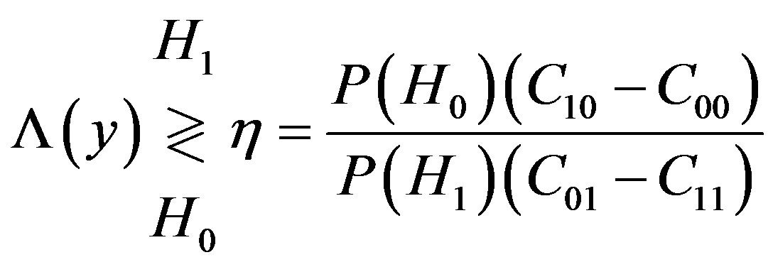 (4)
(4)
the probability , is called a priori probability of
 . When
  the Bayes' test is the maximum aposteriori probability (MAP) test as shown
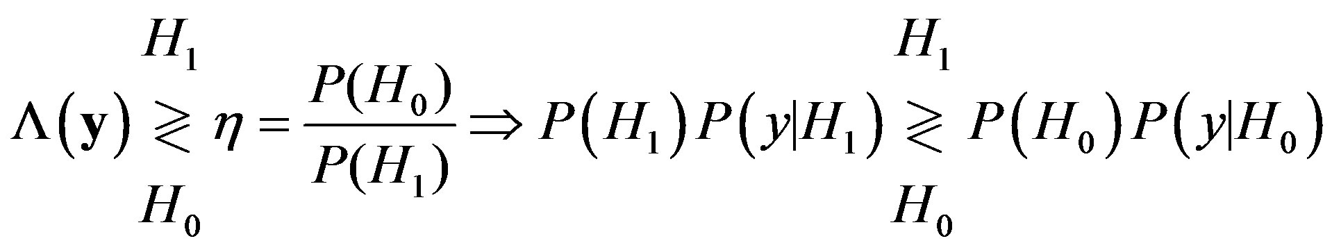 (5)
(5)
Also, when  the MAP test is called maximum-likelihood (ML) test as shown
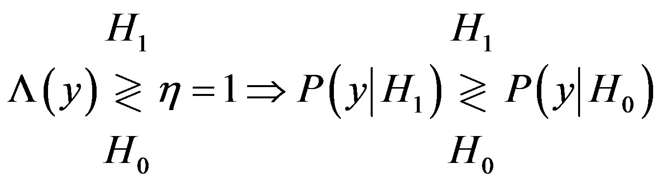 (6)
(6)
2.2. Neyman-Pearson Test
In [12], the NP test follows a different philosophy than that of the Bayes test. The NP test can be expressed in terms of the LRT as
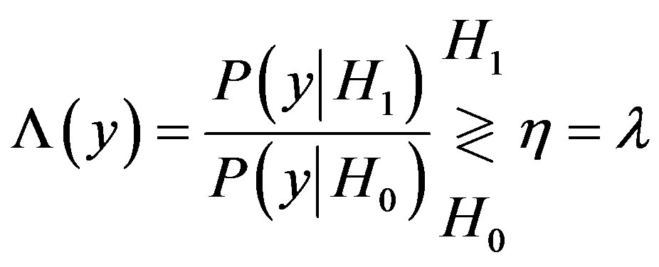 (7)
(7)
where  is the Lagrange multiplier and equals to value of detector threshold.
  is chosen to satisfy the constraint
 (8)
(8)
where  as defined as the type I error or probability of false alarm, which is the probability that the LRT is larger than the threshold when the observation is composed entirely of noise,
  level of significance. The detection is performed on the basis of a Constant False Alarm Rate (CFAR) i.e. The NP technique provides a threshold for detection subject to a constant
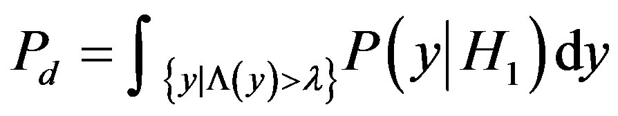
 . The probability of detection can be evaluated as
 (9)
(9)
is the probability that the likelihood ratio is larger than the threshold when the observation is composed of the signal of interest and noise.
If the signal under hypothesis  is assumed to be
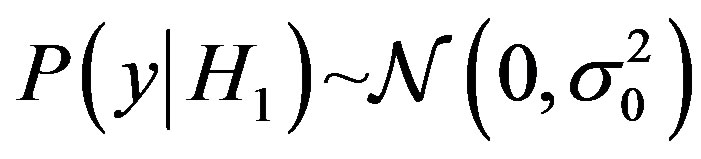 , and under
  is assumed to be
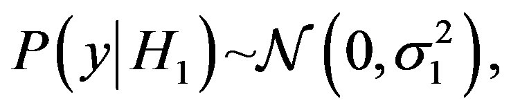
 can be evaluated as
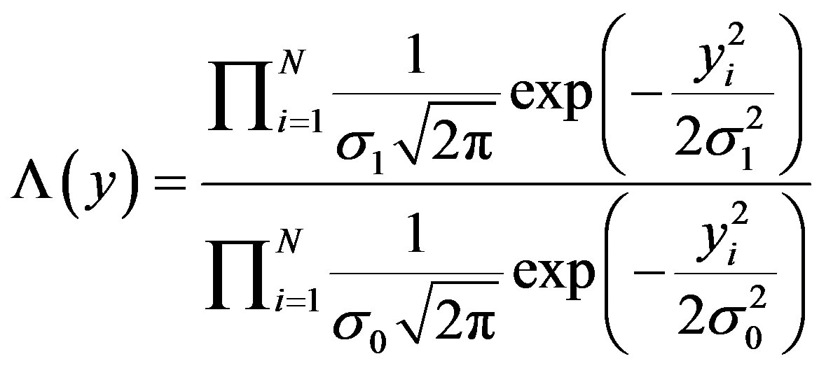 (10)
(10)
taking logarithm, and removing all constants that are independent of vector , and merging with threshold, we obtain
  test as
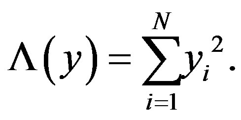 (11)
(11)
Hence, the optimal detector, in the NP sense, is in this case the energy detector.
A test of the hypotheses which is optimal in the NP and Bayes test can be expressed as
 (12)
(12)
3. Previous Works
Energy detector has been widely used for signal detection due to its simple circuit in practical implementation.
The most important preliminary work for the general analysis of energy detector was presented in the landmark paper [10], the authors proposed the model as shown in Figure 1.
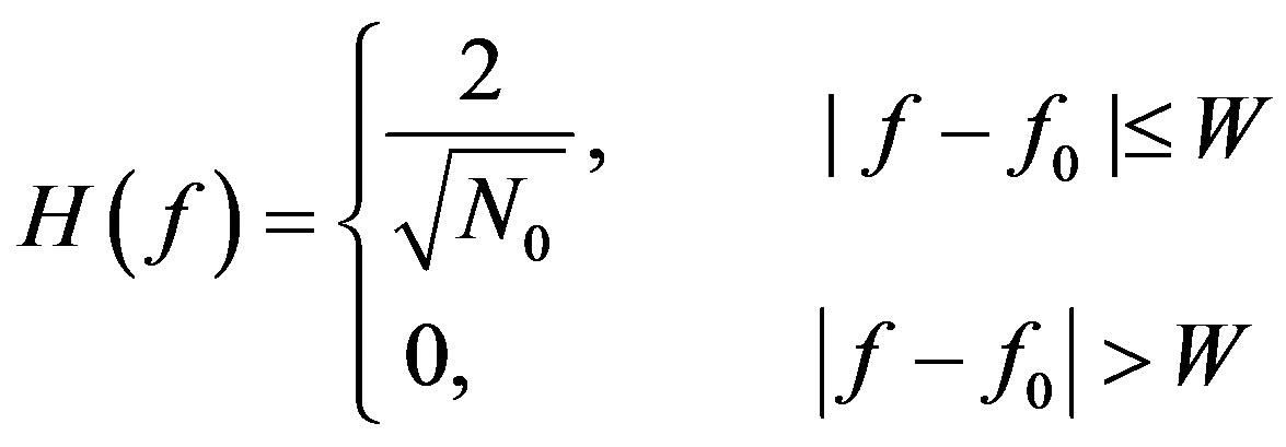
In [10], his classic work was based on detection of a deterministic signal in an additive white Gaussian noise (AWGN), and exact noise variance is known a priori. The input signal  is first passed through an ideal bandpass filter (BPF) with center frequency
  and bandwidth W, with transfer function
 (13)
(13)
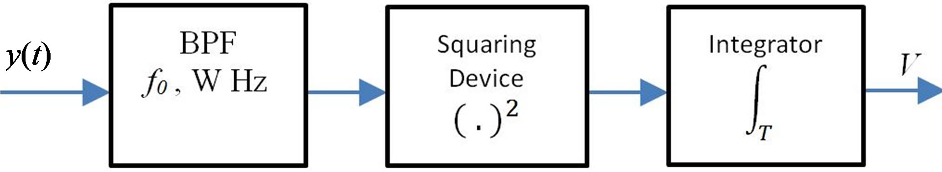
Figure 1. Classical model of energy detector.
where  is the one-sided noise power spectral density, this normalizes it found convenient to compute the false alarm and detection probabilities using the related transfer function. After that the signal squared, and integrated in the observation interval T to produce a test statistic,
  is compared to a threshold
 . The receiver makes a decision that the target signal has been detected if and only if the threshold is exceeded.
In [14], the received signal  of SU under the binary hypotheses testing can be represented as
 (14)
(14)
where  represents the hypothesis corresponding to “no signal transmitted”, and
  to “signal transmitted”,
  is the unknown deterministic transmitted signal, and
  assumed to be an AWGN with zero mean and variance
  is known a priori. The SNR is denoted as
where  variance of signal and
  variance of noise. By using Shannon’s sampling formula, we can obtain the reconstructed noise signal
 (15)
(15)
where
is the normalized  function and
is the i-th noise sample. The test statistic under hypothesis  as follows
 (16)
(16)
If we take the BPF effect and simplify, the decision rule which is employed by the energy detector can be obtained as
 (17)
(17)
The same approach can be applied under hypothesis  when the signal
  is presented, by replacing each
  by
by  where
where
 .
.
The test statistic for both cases can be expressed as
 (18)
(18)
where  chi-square distribution with the
  degree of freedom (DOF), and
  noncentral chi-square distribution with the same number of DOF and a noncentrality parameter equal to
 . The probability of detection and probability of false alarm can be computed if
  by
by
 (19)
(19)
 (20)
(20)
In [15], present several classical models of energy detector, which can be used to evaluate the energy detector performance instead of using the accurate results. These models are easily available for theoretical analysis when one takes advantage of the energy detector for spectrum sensing [16].
In [17], Lehtomaki has done a lot of research work in signal detection based on the ideal energy detector. His main goal was to develop energy based detectors. Different possibilities for setting the detection threshold for a quantized total power energy detector are analyzed.
Energy detector has discussed the existence of signals with random amplitude and channel fading in [18] and [14]. The average probability of detection over a fading channel also derived.
The improved performance of the energy detector for random signals corrupted by Gaussian noise is derived. The derivation is based on a simple modification to the conventional energy detector in [10,14,18] by replacing the squaring operation of the signal amplitude with an arbitrary positive power operation [19].
 (21)
(21)
In [20], in order to solve both the interference avoidance and the spectrum efficiency problem, an optimal spectrum sensing framework is based on the maximum a posteriori probability (MAP) energy detection and its decision criterion based on the primary user activities. The PU activities can be assumed as a two state birthdeath process, death rate  and birth rate
 . Where each transition follows the Poisson arrival process meaning that the length of ON (Busy) and OFF (Idle) intervals of primary network are exponentially distributed. We can estimate the a posteriori probability as follows
 (22)
(22)
 (23)
(23)
where  is the probability of the period used by primary users and
  is the probability of the idle period. From the definition of MAP detection, the detection probability
  and false alarm probability
  can be expressed as follows
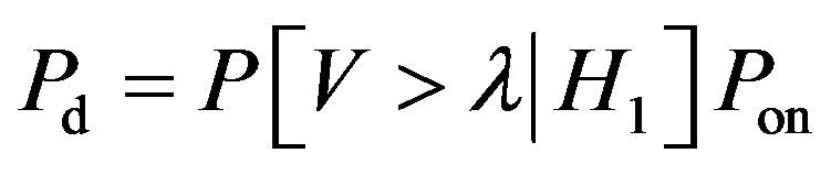 (24)
(24)
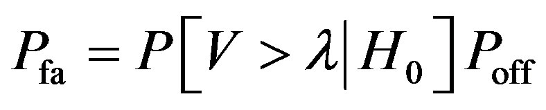 (25)
(25)
where  is a decision threshold of MAP detection.
4. Baseband Energy Detector Model
In practical implementation of the energy detector, transmission and sensing cannot be performed at the same time. Thus, during observation time, all CR users should stop their transmissions. Due to this hardware constraint, CR users should sense the spectrum cyclically with sensing period  and transmission time
 , as described in Figure 2.
A large number of signal processing applications function in real-time systems. Because most signal processing is nowdays implemented with DSP methods, it is suitable for understanding EDs as discrete time (DT) systems. The input signal of the DT system is denoted by a sequence as
 (26)
(26)
where  is analogue continuous time signal that is sampled in order to produce the DT signal
 , the time index n is an integer, and
  is the sampling interval, which is reciprocal to the sampling frequency and is given by
 (27)
(27)
A system model of energy detector with baseband sampling for CR can be shown in Figure 3.
In order to measure the energy of the received signal, the output signal of codec is squared and integrated over
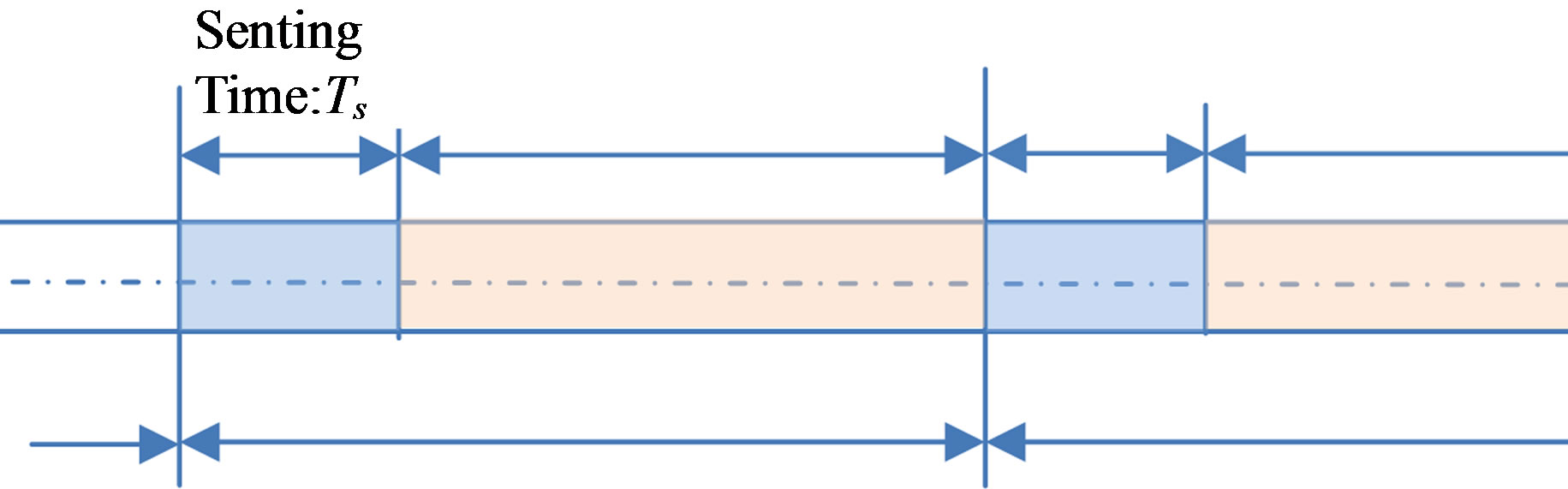
Figure 2. Sensing and transmission structure for energy detector.
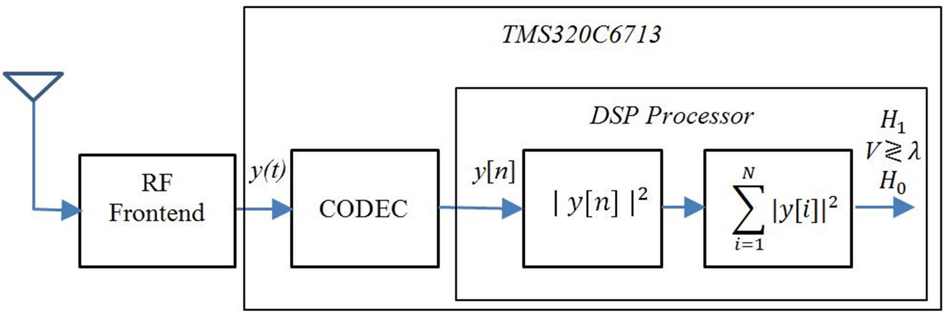
Figure 3. Energy detector with baseband sampling using a DSP kit.
the sensing interval . The sensing interval
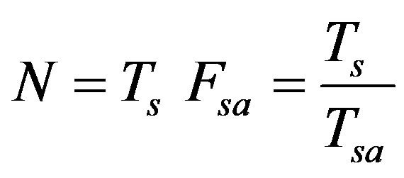
  is usually assumed to be small enough so that the PU signal can span over the whole sensing interval. According to the Nyquist sampling theorem, the minimum sampling rate should be
 , where W is the highest frequency of the original signal, hence, the minimum sample size N collected by the energy detector can be represented as
 . In real-time
  equal to sampling frequency
  of the DSP card, hence as sensing time
  is chosen such that N is an integer
 (28)
(28)
5. Baseband Energy Detector over AWGN Channel
In a binary hypothesis test, the received signal after codec can be given as
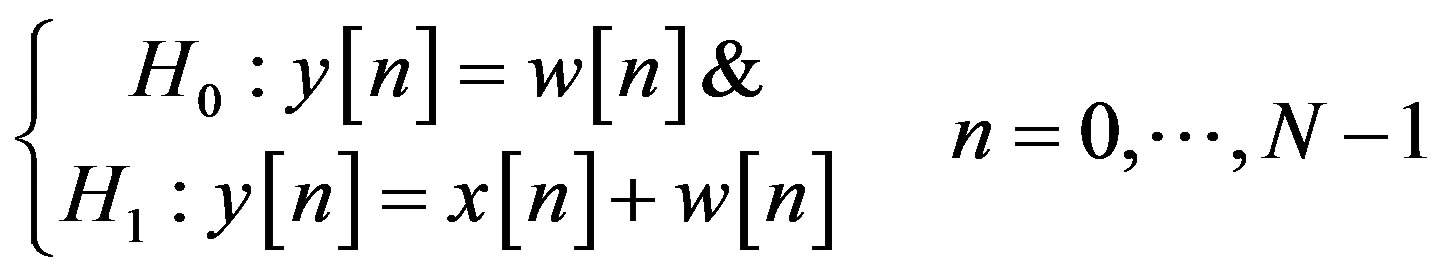 (29)
(29)
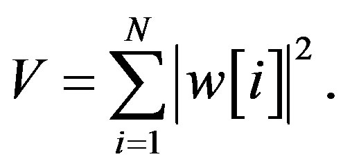
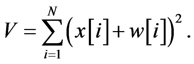
where N denotes the number of samples collected during the signal sensing period. The test statistic for the energy detector with predetermined threshold  is defined as follows
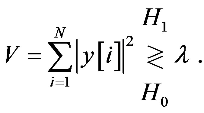 (30)
(30)
When the received signal contains the noise only under  hypothesis, the test statistic can be written as:
 (31)
(31)
Since V is a square sum of N AWGN with zero mean, i.e.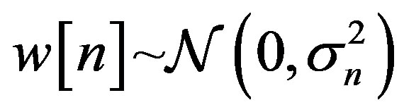 , thus the distribution of the test statistic is a chi-square with N degrees of freedom (DOF)
 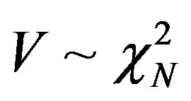 [21], can be evaluated as follows
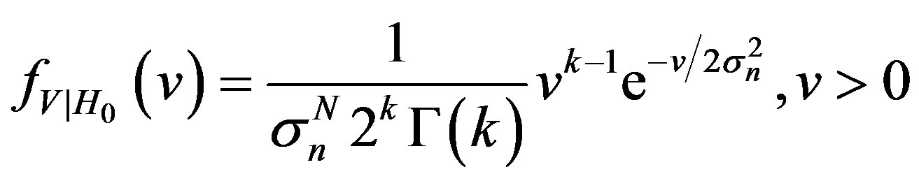 (32)
(32)
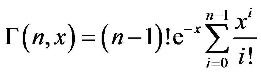
where , is an integer,
  is the gamma function, which is defined as
 [22].
[22].
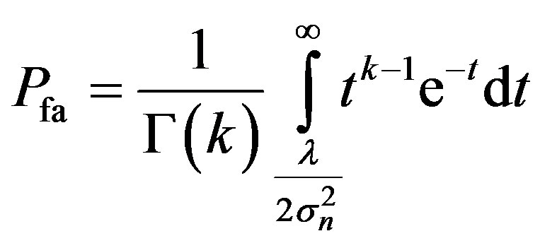
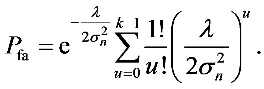
From the definition of false alarm probability, the CR decides in favor of  while the band is idle, thus, the false alarm probability can be expressed as
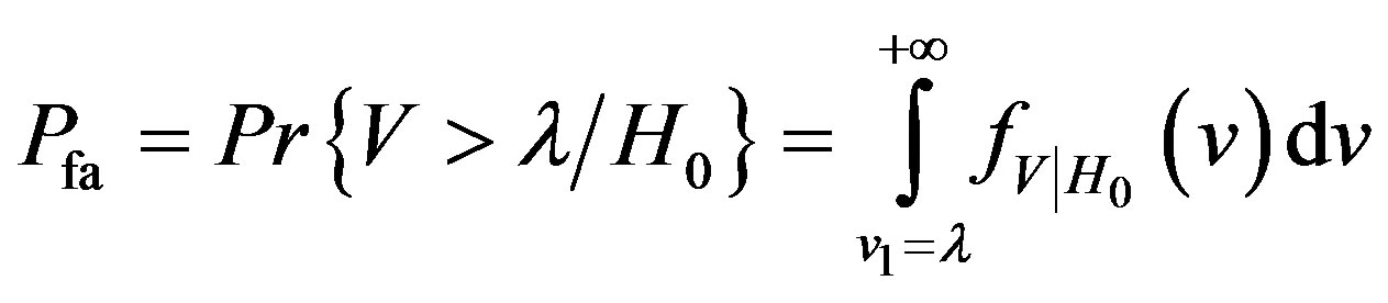 (33)
(33)
 (34)
(34)
To solve this equation, we must apply some variable conversion for  we get
 (35)
(35)
(incomplete gamma functionis given by [22] 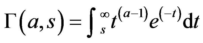 , therefore (35) becomes
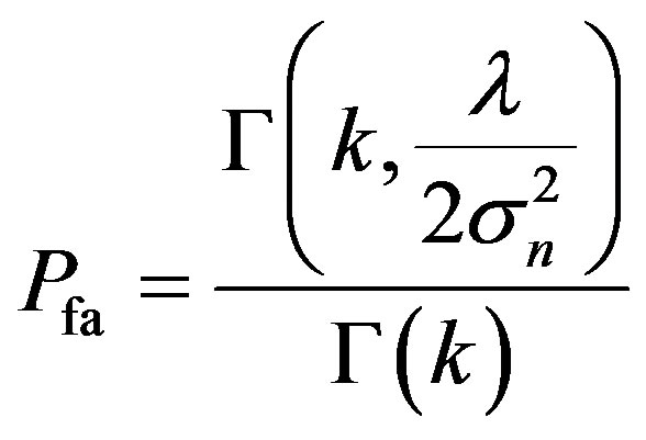 (36)
(36)
In [23, Equation (2.5), p. 24], the incomplete gamma function can be expressed as
 (37)
(37)
based on (37),  can be evaluated as
 (38)
(38)
The same approach is applied when the signal of PU,  is presented hence, the test statistic under hypothesis
  becomes
 (39)
(39)
We can observe that V consists of two terms: a fixed (non-random) component  and a noise component
  obey the Gaussian distribution. More specifically, V is a noncentral chi-square distribution with non-central parameter
 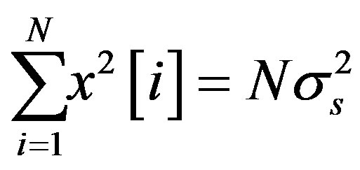 and N DOF,
 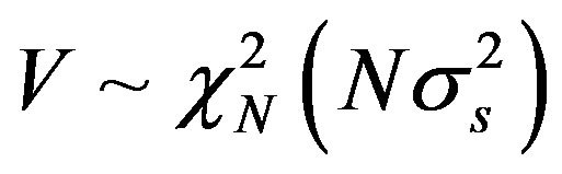 , in particular, the PDFs of V under
  hypothesis takes the form [21]
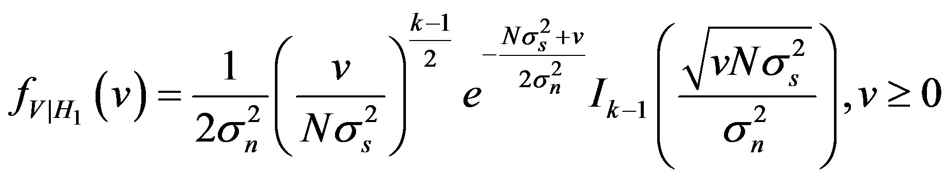 (40)
(40)
where  is the n order modified Bessel function. The probability of detection is
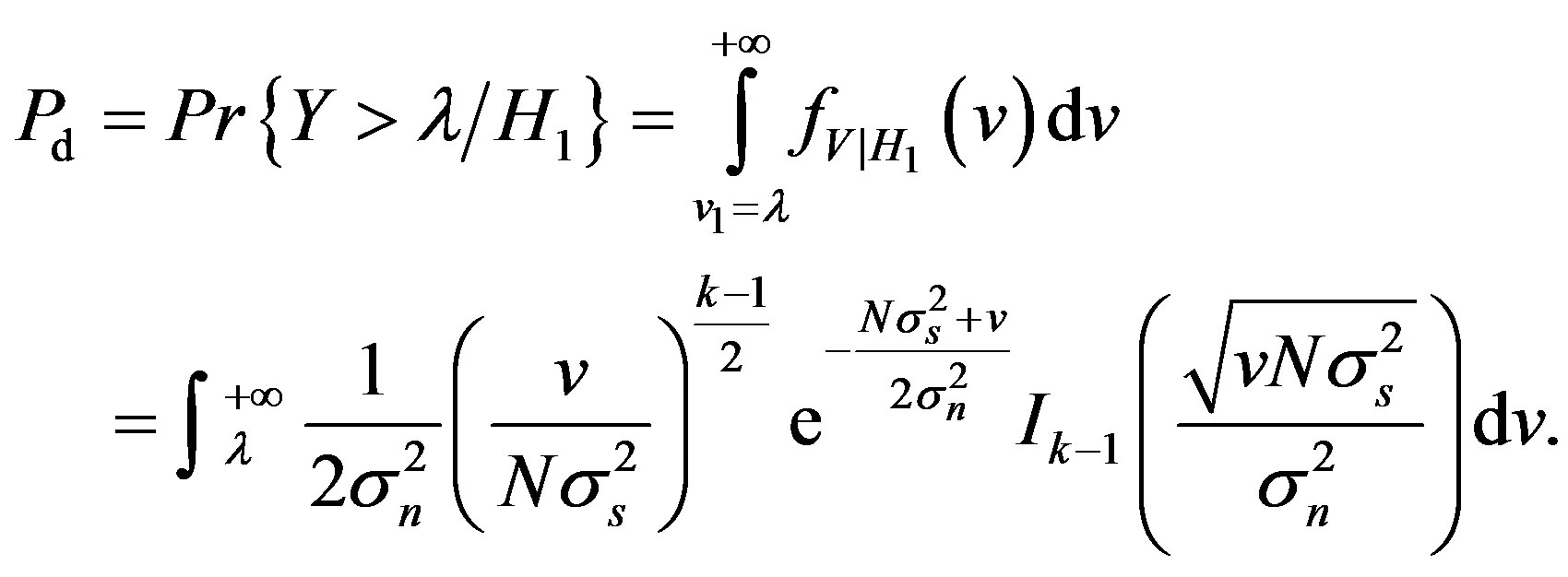 (41)
(41)
The  can be expressed in term of the generalized Marcum Q-function, which is defined as [21]
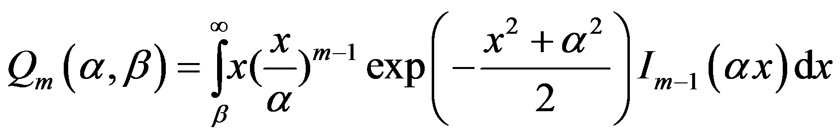 (42)
(42)
Where m is a nonnegative integer, and  and
and  are nonnegative real numbers. If we change variable of integration (41), v to x, where
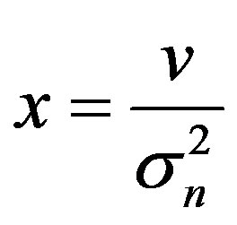 , and let
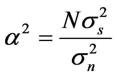 we obtain
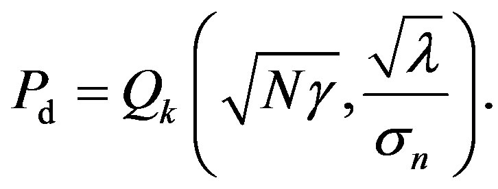 (43)
(43)
If  i.e.
i.e.  the Marcum Q-function is difficult to calculate or to take its inverse, thus, we can use the central limit theorem (CLT), for the large number of sample, we can use the Gaussian distribution to approximate the chi-square distribution, under
  hypothesis, and non-central chi-square distribution, under
  hypothesis, thus, the CLT can therefore be employed to approximate the test statistic as Gaussian
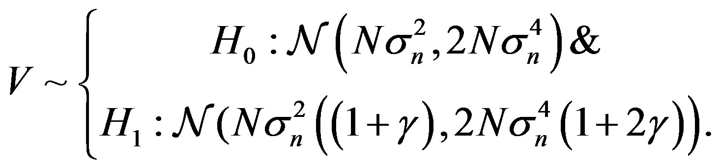 (44)
(44)
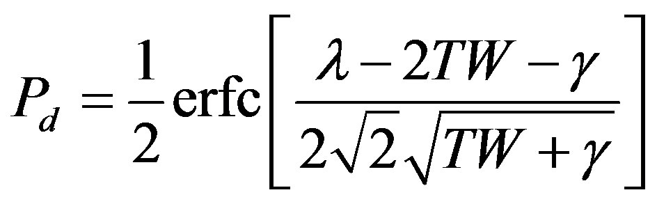
If only AWGN is considered,  and
and  of energy detector can be derived in terms of the Q function as follows
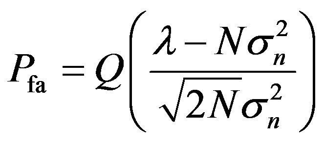 (45)
(45)
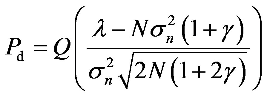 (46)
(46)
where the
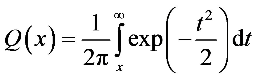
is standard Q-function [22]. The decision threshold  is determined by the pdf of the noise only signal, thus, by using (44), we get
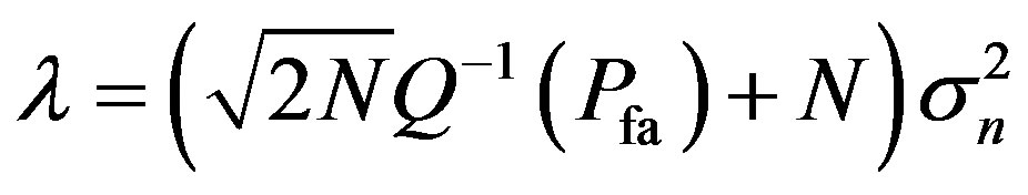 (47)
(47)
where  denote the inverse Q-function [22].
In [20],  should be kept as small and
  should be large as possible to avoid underutilization of transmission opportunities. Note that from (45) and (47), the
  and
and  can be set even without the knowledge of the signal power. The curve represents the performance of the energy detector, which is called the receiver operating curve (ROC), for a given
  pair of
  and
and  representing the point in the ROC. We can plot another curve give an energy detector performance, for a given
  it’s convenient to display the
  with
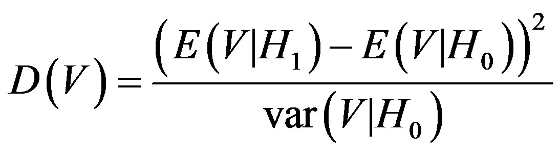
with . In addition to using the ROC curve for performance comparison, one can also resort to the so-called deflection coefficient [12], especially when the statistical properties of the signal and noise are limited to moments up to a given order. The deflection coefficient is defined as
 (48)
(48)
6. Generating Received Signal
The energy detection is used when the CR knows the signal of PU (deterministic) or their probabilities (random). It requires a good model of PU signal and noise is accurately known.
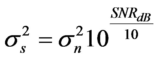
In the process of implementing an energy detector with DSP processor, often we are stymied by the problem of getting a received noisy signal with required amount of SNR i.e. under . To obtain an expression for receiving signals, the PU signal is modeled as being deterministic, by definition of SNR, the variance of signal is
 (49)
(49)
 (50)
(50)
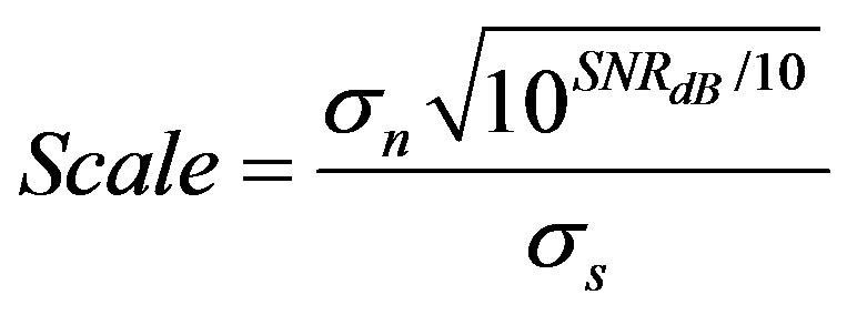
Thus, All we have to do is to scale the signal  appropriately, the received signal expressed as
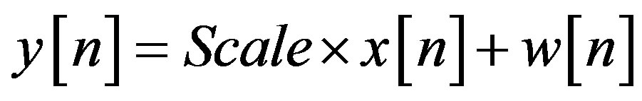 (51)
(51)
Also PU signal can be modeled as being random, the received signal takes the form of a zero mean Gaussian process with known variance 
Most methods for generating white Gaussian noise are based on transformations or operations on white uniform noise. There are several algorithms to generate white uniform noise which is generated by generating a pseudo random number. In this paper, we focus on a particular class of generators suitable for real-time applications. Making choices among generators requires specific criteria. We used two criteria to choose a good generator, are the length of the generation as well as the short implementation period to fit with the real-time environment.
The most widely used techniques for generating pseudo random number have approximately uniform distribution. Such generators, introduced by D. H. Lehmer in 1951, which is known as the linear congruential method [24]
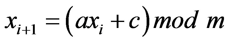 (52)
(52)
m is the nonzero modulus .
.
a is a multiplier .
.
c is an additive constant , The case of
  is called a mixed-congruential generator while
  is referred to as a multiplicative-congruential generator.
 is the starting value, or seed
 .
.
 is the operator means that
  is the residue from dividing
  by m.
by m.
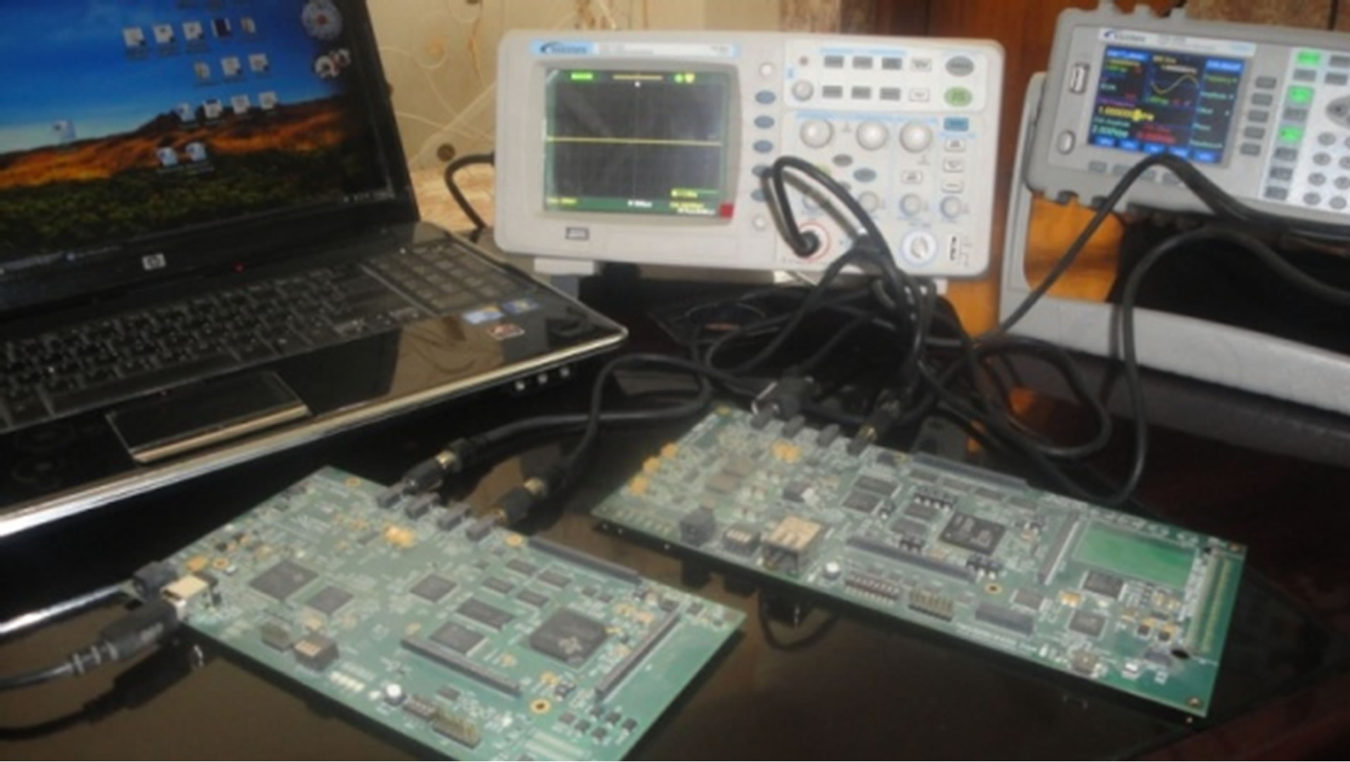
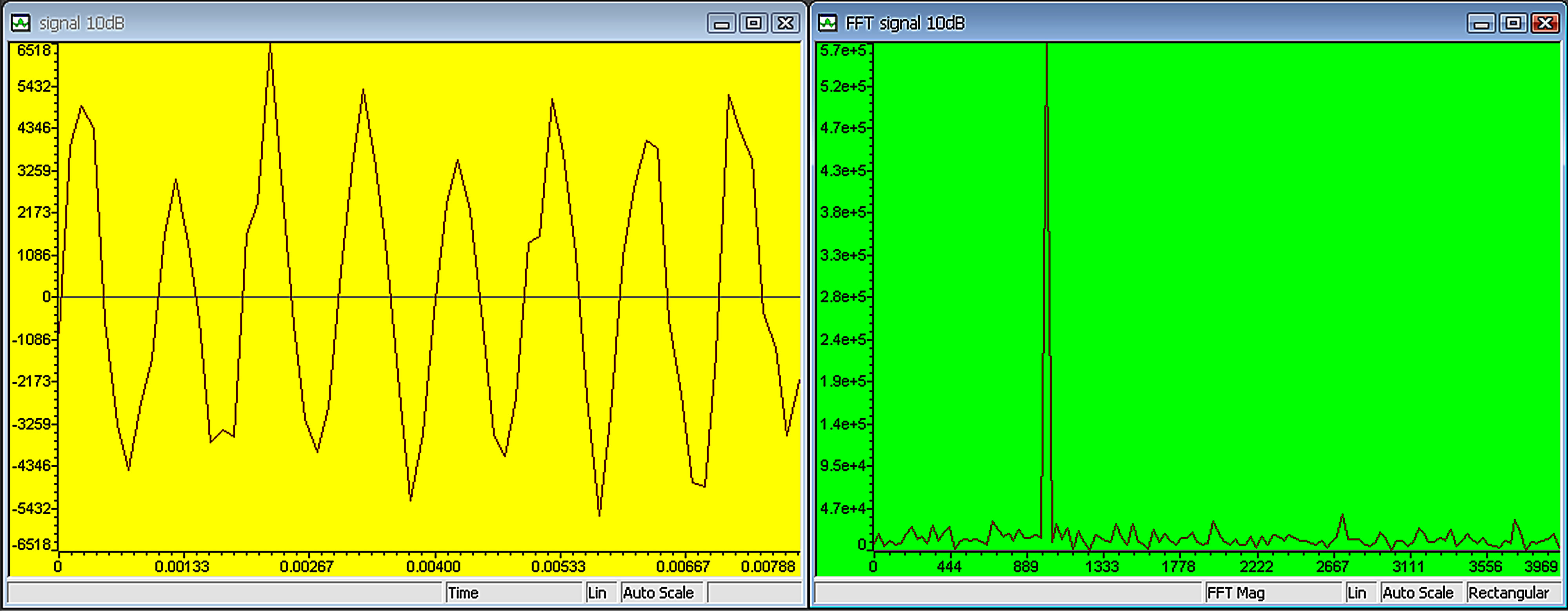
If In [25], many versions of linear congruential generators set the constant c to zero. The resulting multiplicative congruential generator is Park and Miller give suitable choices for The last two algorithms generating white uniform noise zero mean and variance equal to 1/12. In this implementation, we present white Gaussian noise generator based on the CLT (Sum-of-uniforms) method. Therefore, approximation of a white Gaussian noise with zero mean and unit variance, can be gained by realizing the sum of 12 uniform random variables. 7. Implementation of Energy Detector on TMS320C6713 A PU transmitter and SU receiver for CR is implemented on a C6713 DSP board. Figure 4 shows the equipment used in this paper. From (45-47), the energy detector is strongly depending on knowledge of noise power. Thus, accurate estimation of noise power plays an important role in performance of energy detector. We proposed the auxiliary energy detector connected to primary energy detector, which can be used for the detection process of noise power, give an accurate detection as noise power changes. Figure 4. The TMS320C6713 and the equipment. We determined the DSP card cycle numbers of the two algorithms evaluation units to be 392 and 279 respectively, due to this constraint, we are able to fit the algorithm 2 into the signal used under Two scenarios for signal under Figure 5. Time domain representation of Gaussian noise. Figure 6. Time domain and FFT of 10 kHz signal at 5 dB SNR. as as in Figure 7. We use the following implementation parameters: the PU signal Since we set the Figure 9 plots the we take the Fsa at four different values 8, 16, 32 and 96 kHz and and its number of samples 80, 160, 320 and 960 respectively. From the figure it is observed that the detection performance improved by increasing SNR and with increase samples point i.e. sampling frequency. To ensure that the Figure 10 illustrates the values of  and
and  are integers, then this technique will produce a sequence of integers with each integer in the range 0≤xn
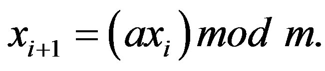 (53)
(53) and
and , this yields a full period generator. The Park Miller generator was implemented using David G. Carta’s optimization which needs only 32 bit integer math, and no division.
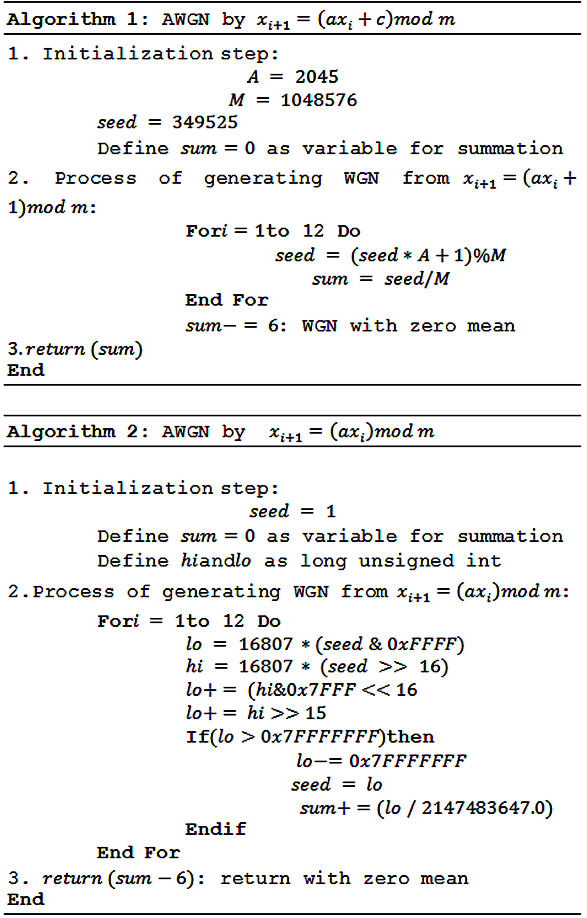
 . Figure 5 shows the time domain plot of white Gaussian noise signal with zero mean and unit variance.
 can be implemented, in (51)
  isa (deterministic) sinusoid signal generated using eight points a table lookup method as in Figure 6, or
  is random, thus,
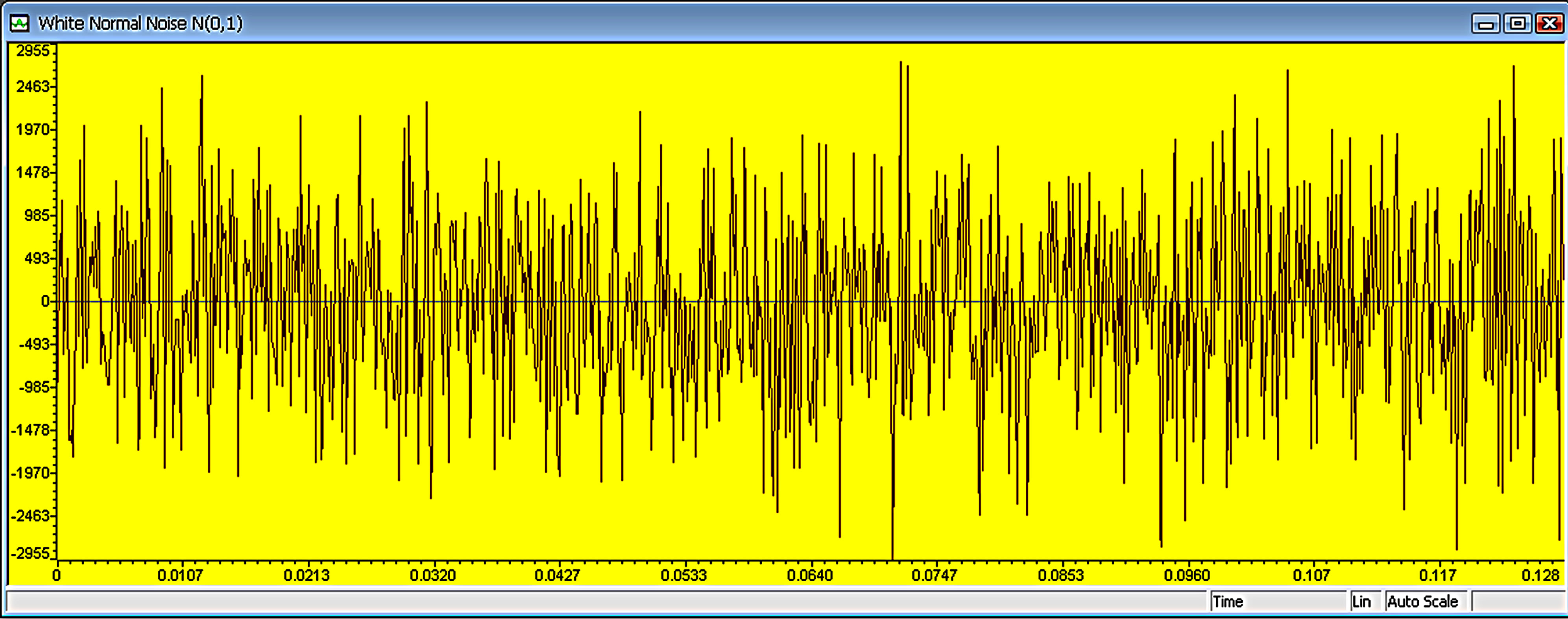
 ,
,  ,
,  and assume
 . The C6713 development board we used has sampling frequencies 8, 16, 32, 44, 1, 48 and
  are supported,
  , we select
 , and
, and 
 , this is to say that we observe test statistic under hypothesis
  for 100 times to yield 99 realizations of detections in theory. We change SNR from –20 dB to 0, and repeat the 100 observations for each to calculate the number of detections. Figure 8 represents 100 observations at –11 dB,
  = 96 kHz it has gotten 4 detections.
 versus SNR.
  can be expressed as [26]
 (54)
(54) is accurately estimated, we will compare the theoretical value and the implementation results. The
  is calculated using the following formula [26]
 (55)
(55) which are calculated for different values of SNRs at
  = 96 kHz. As we know that the estimated value of
  is 0.01, the
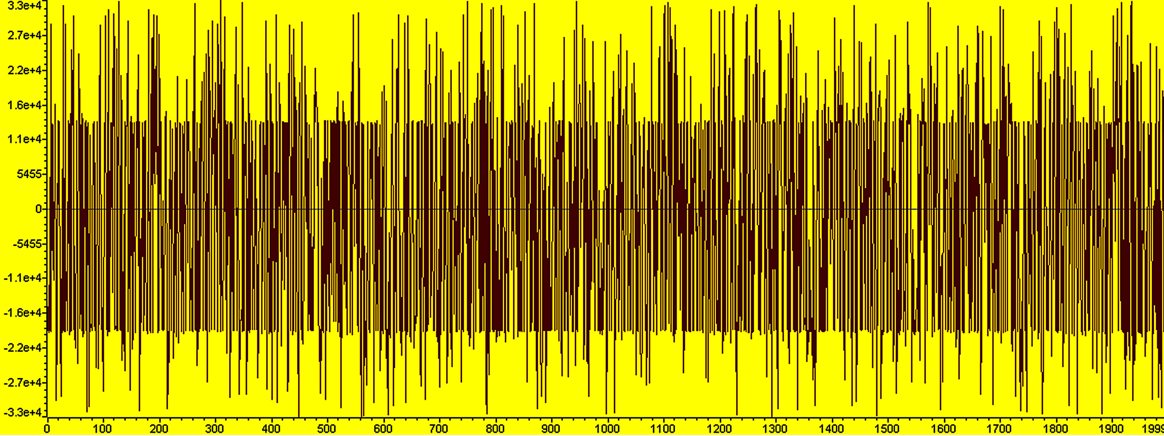
Figure 7. Time domain of 10 kHz signal at −10 dB SNR.
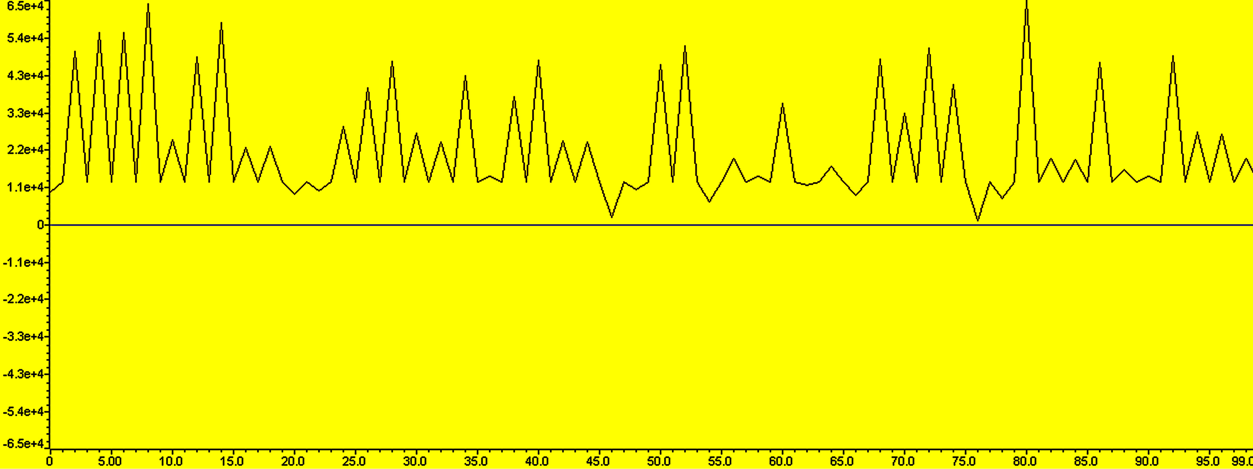
Figure 8. Signal after integrating with 100 frames.
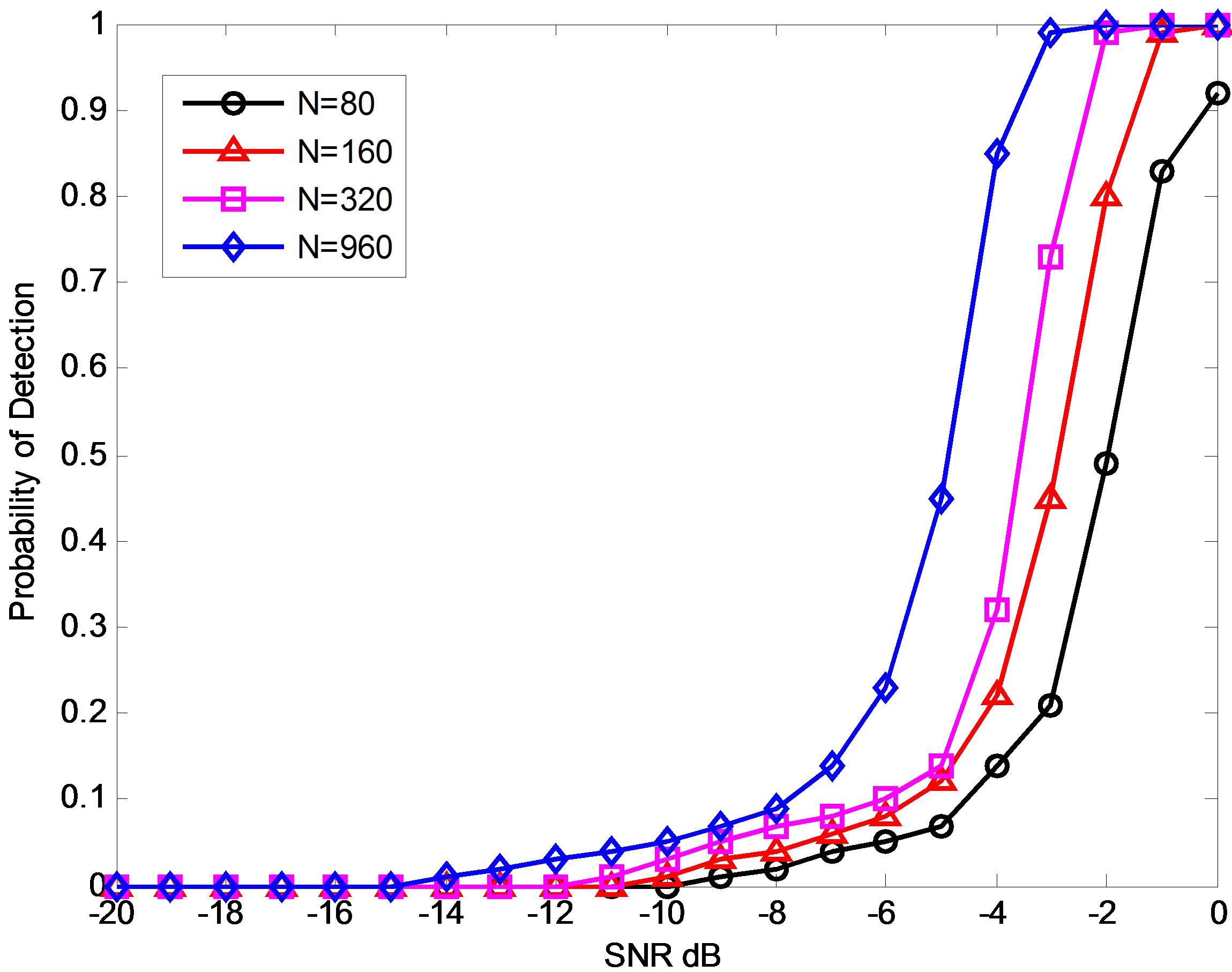
Figure 9. Probability of detection for different SNRs.
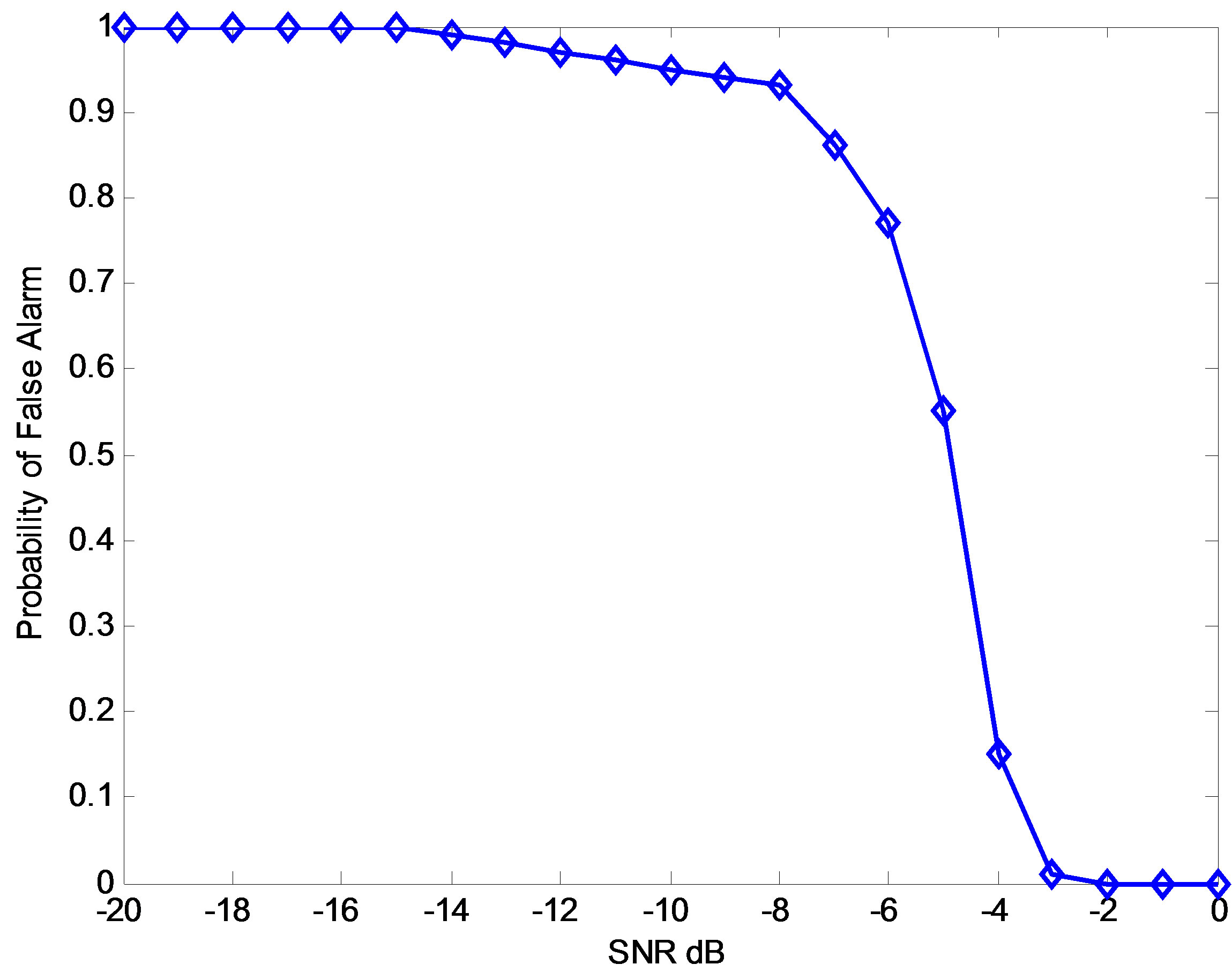
Figure 10.  for different SNRs,
 .
.
figure shows when SNR is between –3 dB and 0, the  = 0.01, 0.0 and 0 which are almost the same and confirm the estimated we used. Thus, it can be concluded when SNR between –3 dB to 0, the energy detector can offer significant detections.
8. Discussion
The energy detector of 100 observations is implemented, the  and
and  are calculated.
  is different from the estimated value. The SNR plays an important factor that influences the detections. By changing the value of the SNR from –20 to 0 dB, we get the relationship between the SNR and the detections Figure 9, from that figure, we can see from –3 dB to 0, the energy detector gives best performance. We also calculate the relation between SNR and
  as, as shown in Figure 10.
9. Conclusion
The energy detection is worldwide in the sense that it can detect any type of signal, and does not need any knowledge about the signal to be detected. Moreover, the noise power needs to be known to set the determination threshold. The main advantages of energy detection based spectrum sensing are its simplicity, low computational and implementation costs as well as its ability to work regardless of the actual signal to be detected. In the present work, without involving the sampling theorems and the accompanying approximation, we derive the expressions for probability of detection and false alarm over AWGN. Therefore, the calculation is progressively precise. Also, the performance of the energy detector in real-time is analyzed.
10. Acknowledgements
We would like to appreciate the valuable assistance of Dr. Deah J. Kadhim and Dr. Tarik Z. Ismaeel at the electrical engineering department.
REFERENCES
- I. F. Akyildiz, W. Y. Lee, M. C. Vuran and S. Mohanty, “Next Generationdynamic Spectrum Access/Cognitive Radio Wireless Networks: A Survey,” Computer Networks, Vol. 50, No. 13, 2006, pp. 2127-2159. doi:10.1016/j.comnet.2006.05.001
- S. Haykin, “Cognitive Radio: Brain-Empowered Wireless Communications,” IEEE Journal on Selected Areas in Communications, Vol. 23, No. 2, 2005, pp. 201-220. doi:10.1109/JSAC.2004.839380
- D. Cabric, S. M. Mishra, D. Willkomm, R. W. Brodersen and A. Wolisz, “A Cognitive Radio Approach for Usage of Virtual Unlicensed Spectrum,” Proceedings of 14th IST Mobile and Wireless Communications Summit, 2005.
- W. Zhang, R. Mallik and K. Letaief, “Optimization of Cooperative Spectrum Sensing with Energy Detection in Cognitive Radio Networks,” IEEE Transactions on Wireless Communications, Vol. 8, No. 12, 2009, pp. 5761- 5766.
- H. P. Zhiquan, S. G. Cui and A. Sayed, “Collaborative Wideband Sensing for Cognitive Radios,” IEEE Signal Processing Magazine, Vol. 25, No. 6, 2008, pp. 60-73. doi:10.1109/MSP.2008.929296
- D. Cabric, S. M. Mishra and R. W. Brodersen, “Implementation Issues in Spectrum Sensing for Cognitive Radios,” Proceedings of Asilomar Conference on Signals, Systems and Computers, Pacific Grove, 7-10 November 2004, pp. 772-776.
- W. A. Gardner, A. Napolitano and L. Paura, “Cyclostationarity: Half a Century of Research,” Signal Processing, Vol. 86, No. 4, 2006, pp. 639-697. doi:10.1016/j.sigpro.2005.06.016
- D. Cabric, S. M. Mishra and B. W. Brodersen, “Implementation Issues in Spectrum Sensing for Cognitive Radios,” Berkeley Wireless Research Center, University of California, Berkeley, 2004.
- P. Pawetczak, G. J. M. Janssen and R. V. Prasad, “Performance Measures of Dynamic Spectrum Access Networks,” IEEE Global Telecommunications Conference, San Francisco, 27 November -1 December 2006, pp. 1-6.
- H. Urkowitz, “Energy Detection of Unknown Deterministic Signals,” Proceedings of the IEEE, Vol. 55, No. 4, 1967, pp. 523-531. doi:10.1109/PROC.1967.5573
- L. L. Scharf, “Statistical Signal Processing: Detection, Estimation and Time Series Analysis,” Addison-Wesley, Reading, 1991.
- S. M. Kay, “Fundamentals of Statistical Signal Processing: Detection Theory,” 1st Edition, Prentice-Hall, Upper Saddle River, 1998.
- H. V. Poor, “An Introduction to Signal Detection and Estimation,” Springer, New York, 1994.
- F. F. Digham, M. S. Alouini and M. K. Simon, “On the Energy Detection of Unknown Signals over Fading Channels,” IEEE Transactions on Communications, Vol. 5, No. 1, 2003, pp. 3575-3579.
- R. F. Mills and G. E. Prescon, “A Comparison of Various Radiometer Detection Models,” IEEE Transactions on Aerospace and Electronic Systems, Vol. 32, No. 1, 1996, pp. 467-473. doi:10.1109/7.481289
- S. Ciftci and M. Torlak, “A Comparison of Energy Detectability Models for Spectrum Sensing,” Proceedings of IEEE Global Telecommunications Conference, New Orleans, 30 November-4 December 2008, pp. 1-5.
- J. J. Lehtomaki, “Analysis of Energy Based Signal Detection,” A Doctoral Dissertation, University of Oulu, Oulu, 2005. http://herkules.oulu.fi/isbn9514279255
- V. I. Kostylev, “Energy Detection of a Signal with Random Amplitude,” IEEE International Conference on Communications, New York, May 2002, pp. 1606-1610.
- Y. Chen, “Improved Energy Detector for Random Signals in Gaussian Noise,” IEEE Transactions on Wireless Communications, Vol. 9, No. 2, 2010, pp. 558-563. doi:10.1109/TWC.2010.5403535
- W.-Y. lLee and I. F. Akyildiz, “Optimal Spectrum Sensing Framework for Cognitive Radio Networks,” IEEE Transactions on Wireless Communications, Vol. 7, No. 10, 2008, pp. 3845-3857.
- J. G. Proakis, “Digital Communications,” 4th Edition, McGraw-Hill, New York, 2001.
- I. S. Gradshteyn and I. M. Ryzhik, “Table of Integrals, Series, and Products,” 7th Edition, Academic, San Diego, 2007.
- J. J. Lehtomaki, “The Detection and Correlation Modeling of Rayleigh Distribution Radar Signal,” A Master Dissertation, Air Force Institute of Technology, University of Air, 1992. www.dtic.mil/cgi-bin/GetTRDoc?AD=ada256612
- W. H. Press, S. A. Teukolsky, W. T. Vetterling and B. P. Flannery, “Numerical Recipes in C,” Cambridge University Press, Cambridge, 2002.
- D. Carta, “Two Fast Implementations of the Minimal Standard Random Number Generator,” Communications of the ACM, Vol. 33, No. 1, 1990, pp. 87-88. doi:10.1145/76372.76379
- http://www.radartutorial.eu/18.explanations/ex10.en.html