Communications and Network
Vol.3 No.2(2011), Article ID:4972,5 pages DOI:10.4236/cn.2011.32013
On Time-of-Arrival Statistic of Gaussian Channel Model
Wireless Technologies Department, Mera NN, Russia
E-mail:{flak, ave, ermol}@mera.ru
Received March 23, 2011; revised April 20, 2011; accepted April 30, 2011
Keywords: Multipath Channels, Channel Modeling, Scattering, Time-of-Arrival, Angle-of-Arrival, Spatial Correlation, Gaussian
Abstract
A model of an angle-spread source, termed the “Gaussian Channel Model” is considered. The cumulative distribution function of the Time-of-Arrival of the multipath components is derived for an arbitrary angle spread. The simple approximate expressions for the Time-of-Arrival cumulative distribution function and probability density function are proposed. Numerical results obtained with the help of the derived expressions show the good coincidence with the experimental data and other known results.
1. Introduction
The implementation of smart antennas at base stations (BS) gives the opportunity to significantly enhance the performance of wireless networks [1]. The plenty of algorithms for adaptive array signal processing have been proposed and investigated (see for example, [2,3]). The effectiveness of these algorithms depends on the behavior of the signal propagation channel. Therefore, accurate statistical channel models are required for the validation of these adaptive algorithms.
The propagation channel can be model in many ways. The one of the most popular strategies is “geometric modeling” [4]. It idealizes the multipath propagation environment via a geometric abstraction of the spatial relationships among the transmitter, the receiver and the scatterers. In other words, geometric models map the propagation channel’s geometry into the measurable fading metrics. The metrics of interest, as a rule, are the Angle-of-Arrival (AoA) distribution, the Time-of-Arrival (ToA) distribution, the power azimuth spectrum (PAS) and the power delay spectrum (PDS).
There exist various geometric models based on a different idealization of the propagation channel’s geometry. The corresponding highlights and comparisons can be found in reviews [4,5]. The modeling approach implying a Gaussian density of scatterers centered at the transmitter can be considered as both effective and safe (i.e. well fitting the experimental data in the most of cases) [4]. The fundamental framework on the channel modeling under assumption of the Gaussian scattering was provided in [6].
In [7,8], the Gaussian distribution of scatterers was used to model the urban macrocellular environment and the “Gaussian Channel Model” (GCM) was proposed. This model assumes that the scatterers can be situated in any point in the horizontal plane and the probability of occurrence of the scatterer location decreases in accordance with a Gaussian law when its distance from the user equipment (UE) increases. This results in a situation when the BS “sees” the UE as a source with some angular distribution. As follows from the presented results, the AoA probability density function (pdf) for the GCM fits the experimental data [9] well.
The goal of this paper is to give the further elaboration to the GCM. In order to characterize the temporal dispersion of the signal seen by the BS, the ToA distribution is derived.
This paper is organized as follows: Section 2 gives the brief background on the GCM and derives the strict expression for the ToA cumulative distribution function (cdf). Section 3 introduces the approximate expression for ToA cdf and derives the ToA pdf. The comparison of the derived ToA distribution with the known results and the measured data is performed. Section 4 concludes the main findings of the paper.
2. ToA CDF
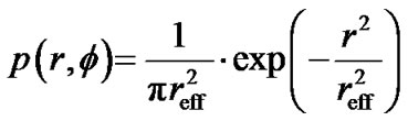
The GCM assumes that the random scatterers are centered at the transmitter (UE) and the probability of scatterer’s appearance decreases away from the transmitter location. In a polar coordinate system the corresponding distribution can be written as [7]:
 (1)
(1)
where r is the distance between the scatterer and the UE, j is the azimuth angle, reff is the nominal distance at which the pdf (1) decreases by e times, i.e. p(reff, j ) = e−1 p(0,j ). It can be noted that the marginal pdf p(j ) is uniform, i.e., the scatterers’ density is independent of azimuth direction.
Figure 1 gives the background on the geometry of the GCM. It is supposed that D is the line-of-sight (LoS) distance between the UE (transmitter) and the BS (receiver), (x,y) are the Cartesian coordinates centered at the UE, qeff is the angle corresponding to the radius reff seen by the BS.
The signal transmitted by the UE is coming to the BS via different paths so the BS receives a set of signals having different AoAs and ToAs. To get the ToA distribution, we will exploit some geometrical relationships and the fact that the distance traveled by the radio signal defines its propagation delay.
Let 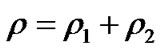 be the sum of the distances from an arbitrary scatterer to the BS and the UE, correspondingly. It is known that the locus of points with the same value of distance r is an ellipse. The BS and the UE are situated at the focuses of the ellipse and the lengths of its semi-axes are related though Equations
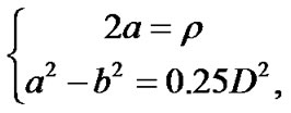 (2)
(2)
where a and b are the lengths of major and minor semi-axis (see Figure 1).
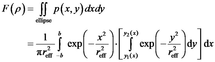
The distance traveled by a signal via any scatterer (lying inside the ellipse) varies in the range of (D…r ). To derive the distribution of value r we should find the probability F(r) of the scatterer appearance within the ellipse boundaries.
Taking into account (1), the probability is given as
 (3)
(3)
where the functions y1(x) and y2(x) define the ellipse boundaries subject to (2):
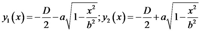 (4)
(4)
It is possible to simplify (3) by introducing the new variables u = , v =
, v = . After the substitution, the equation (3) takes form
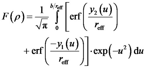 (5)
(5)
Given the speed of light equals c, the distance r causes the propagation delay t = . As follows from Figure 1, r = D is the shortest distance between the transmitter and receiver. This means that the minimum propagation delay is equal to t0 =
 . Considering the normalized propagation delay tn =
  and the effective diameter d =
  =
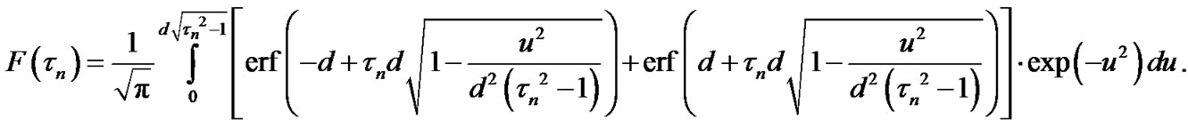
= , the Equation (5) can be rewritten as Equation (6).
The Equation (6) represents the exact expression for the ToA cdf. Unfortunately, this dependence has too complex form and its practical usage is difficult. Therefore, it is of interest to introduce a simpler formula.
3. The Approximation of the ToA Distribtion
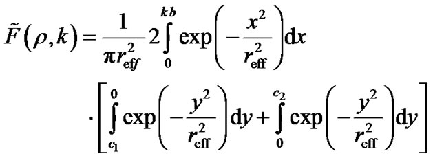
The Equation (3) corresponds to the strict approach when the probability of the scatterer’s appearance within the ellipse boundaries is to be found. Let us now replace the ellipse boundaries with rectangular ones. In such a case the double integral in (3) can be written as a product of two one-dimensional integrals, i.e.
 (7)
(7)
where c1 = −0.5D-a, c2 = −0.5D + a are the limits of integration over the variable y, k is the additional parameter introduced to minimize the approximation error due to the boundary replacement.
 (6)
(6)
Taking into account (5) and (6), it is straightforward to obtain
 (8)
(8)
The Equation (8) can be rewritten as
 (9)
(9)
To minimize the difference between the exact (6) and approximate (9) expressions it is convenient to find the extremum of the mean-root-square error e considering k as a variable subject to the fixed parameter qeff
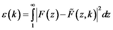 (10)
(10)
The solution of (10) has been found numerically. The result is plotted in Figure 2 as the dependence of k upon qeff (the dotted curve). This dependence allows analytical approximation with the help of Equation
 (11)
(11)
The function (11) is presented in Figure 2 as the solid curve. It is clear to see that in the range of qeff = 0…30˚ the chosen approximation fits the numerical solution quite well.
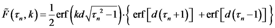
The substitution of (11) into (9) results in expression
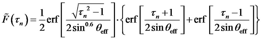 (12)
(12)
In the macrocellular environment the angular spread is rather moderate so that the value of qeff is less than 30˚. Hence, sinqeff is less than 0.5 and the inequality
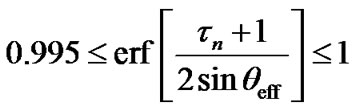 (13)
(13)
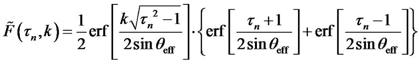
takes place for all values of tn . Therefore, (12) can be reduced to the form
 (14)
(14)
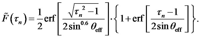
The Equation (14) represents the approximate expression for the ToA cdf. To compare it with the exact formula (6), Figure 3 shows cdfs F(tn) and  for the different values of θeff = 5˚; 15˚; 30˚ and 45˚. The solid and dash curves correspond to (6) and (14), respectively.
One can see that the approximate cdfs fit the exact ones quite well. Therefore, (14) may be used to model temporal dispersion of the signal received by the BS.
Sometimes the usage of a pdf instead of a cdf is more convenient. Performing the derivation of (14) by variable tn, one can obtain that the corresponding ToA pdf is given as
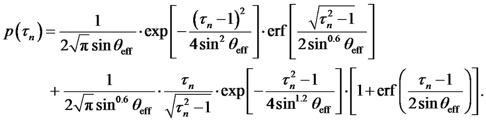 (15)
(15)
The obtained results can be validated by means of comparison with other known results. In [10], the detail study of the standard Gaussian and hyperbolic channel models is presented. Among other results, it defines the ToA pdf of the Gaussian scatterer distribution as
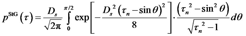 (16)
(16)
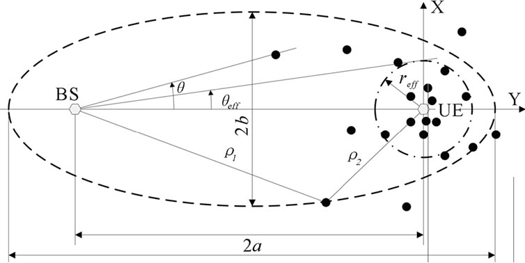
Figure 1. The geometry of the Gaussian channel model.

Figure 2. Parameter k versus qeff (dotted curve-numerical solution, solid curve-approximation).
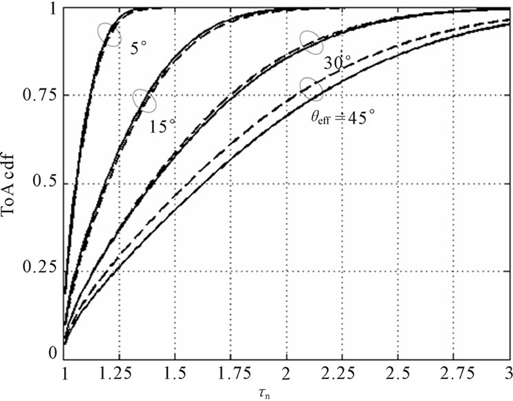
Figure 3. The comparison of the exact (solid curves) and approximate (dash curves) ToA cdfs.
To the end of comparison, Equations (15) and (16) are plotted against tn in Figure 4 as the solid and dash-dot curves, correspondingly. In accordance with [10], the parameter DS is set to 5. The parameter qeff in (15) is chosen to provide the best fitting and equals to 16˚. To realize the comparison with the hyperbolic scatterer distribution, Figure 4 also shows the corresponding ToA pdf with the parameter Db = 5 (dash curve).
Besides the comparison with the known theoretical Equations, the validation of the obtained results against the experimental data is of interest. Some experimental data can be found in literature. For example, [9] presents the results of the measurement campaigns conducted to collect information about the temporal and azimuthal signal dispersions. To depict the temporal dispersion seen in the typical urban environment the histogram of estimated delays is given. The corresponding ‘measured’ pdf produced from that histogram is plotted in Figure 4 as the set of “·” points.
As follows from Figure 4, the distribution (15) is satisfactorily overlapped with other theoretical results and fits the experimental data quite well.
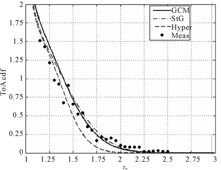
Figure 4. The GCM, standard gaussian, standard hyperbolic and experimental ToA pdfs.
As follows from Figure 4, the distribution (15) is satisfactorily overlapped with other theoretical results and fits the experimental data quite well.
4. Conclusions
In this paper the further elaboration of the Gaussian Channel Model has been performed. This model is suitable for representing the signal seen at the BS in the urban macrocellular environment, and assumes that the probability of the scatterer occurrence decreases in accordance with a Gaussian law when its distance from the UE antenna increases. In order to characterize the temporal dispersion of the signal seen by the BS, the exact expression for the ToA cdf has been derived. To simplify the form of the ToA distribution an approximate approach has been considered and the simpler expressions for the ToA cdf and pdf have been proposed. The comparison of the obtained pdf with the published experimental results shows a good agreement.
5. References
[1] L. C. Godara, “Applications of Antenna Arrays to Mobile Communications, Part I: Performance Improvement, Feasibility, and System Considerations,” Proceedings of the IEEE, Vol. 85, No. 7, 1997, pp. 1031-1060. doi:10.1109/5.611108
[2] J. B. Andersen, “Antenna Arrays in Mobile CommunicaTions: Gain, Diversity, and Channel Capacity,” IEEE Antennas and Propagation Magazine, Vol. 42, No. 2, 2000, pp. 12-16. doi:10.1109/74.842121
[3] L. C. Godara, “Application of Antenna Arrays to Mobile Communications, Part II: Beam-Forming and Direction-of-Arrival Considerations,” Proceedings of the IEEE, Vol. 85, No. 8, 1997, pp. 1195-1245. doi:10.1109/5.622504
[4] K. T. Wong, Y. I. Wu and M. Abdulla, “Landmobile Radiowave Multipaths’ DOA Distribution: Assessing Geometric Models by the Open Literature’s Empirical Datasets,” IEEE Transactions on Antennas and Propagation, Vol. 58, No. 3, 2010, pp. 946-958. doi:10.1109/TAP.2009.2037698
[5] R. B. Ertel, P. Cardieri, K. W. Sowerby, T. S. Rappaport and J. H. Reed, “Overview of Spatial Channel Models for Antenna Array Communication Systems,” IEEE Personal Communications, Vol. 5, No. 1, February 1998, pp. 10-22. doi:10.1109/98.656151
[6] R. Janaswamy, “Angle and Time of Arrival Statistics for the Gaussian Scatter Density Model,” IEEE Transactions on Wireless Communications, Vol. 1, No. 3, 2002, pp. 488-497. doi:10.1109/TWC.2002.800547
[7] D. D. N. Bevan, V. T. Ermolayev, A. G. Flaksman and I. M. Averin, “Gaussian Channel Model for Mobile Multipath Environment,” EURASIP Journal on Applied Signal Processing, Vol. 2004, No. 9, 2004, pp. 1321-1329. doi:10.1155/S1110865704404028
[8] D. D. N. Bevan, V. T. Ermolayev, A. G. Flaksman, I. M. Averin and P. M. Grant, “Gaussian Channel Model for Macrocellular Mobile Propagation,” Proceedings of 13th European Signal Processing Conference, Antalya, 4-8 September 2005.
[9] K. I. Pedersen, P. E. Mogensen and B. H. Fleury, “A Stochastic Model of the Temporal and Azimuthal Dispersion Seen at the Base Station in Outdoor Propagation Environments,” IEEE Transactions on Vehicular Technology, Vol. 49, No. 2, 2000, pp. 437-447. doi:10.1109/25.832975
[10] K. N. Le, “On Angle-of-Arrival and Time-of-Arrival Statistics of Geometric Scattering Channels,” IEEE Transactions on Vehicular Technology, Vol. 58, No. 9, 2009, pp. 4257-4264. doi:10.1109/TVT.2009.2023255