Received 9 February 2015; accepted 23 February 2015; published 26 February 2015

ABSTRACT

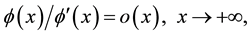
We call “asymptotic mean” (at +∞) of a real-valued function the number, supposed to exist, , and highlight its role in the geometric theory of asymptotic expansions in the real domain of type (*)where the comparison functions, forming an asymptotic scale at +∞, belong to one of the three classes having a definite “type of variation” at +∞, slow, regular or rapid. For regularly- varying comparison functions we can characterize the existence of an asymptotic expansion (*) by the nice property that a certain quantity has an asymptotic mean at +∞. This quantity is defined via a linear differential operator in f and admits of a remarkable geometric interpretation as it measures the ordinate of the point wherein that special curve, which has a contact of order n − 1 with the graph of f at the generic point t, intersects a fixed vertical line, say x = T. Sufficient or necessary conditions hold true for the other two classes. In this article we give results for two types of expansions already studied in our current development of a general theory of asymptotic expansions in the real domain, namely polynomial and two-term expansions.

Keywords:

Asymptotic Expansions, Formal Differentiation of Asymptotic Expansions, Regularly-Varying and Rapidly-Varying Functions, Asymptotic Mean

1. Introduction

In our current endeavor to establish a general analytic theory of asymptotic expansions in the real domain [1] -[6] , we highlighted that what we called the geometric approach leads in a natural way to a linear differential operator, say, depending solely on the comparison functions appearing in a possible expansion; certain asymptotic or integral conditions involving the quantity then characterize an expansion of a given function f either in itself or matched to other expansions obtained by formal differentiation in suitable senses. The theory we are referring to is based on the following ideas. Suppose one wishes to find conditions (sufficient and/or necessary) for the validity of an asymptotic expansion

(1.1)

where the ordered n-tuple of comparison functions forms an asymptotic scale at +∞, that is to say: i.e.. In this paper we intentionally choose as this is the situation wherein the classical concept of asymptotic mean plays a role. The simplest elementary case is that of an “asymptotic straight line”―,―and it goes back to Newton the “natural” idea of looking at this contingency as the “limit position of the tangent line at the graph of f” as the point of tangency goes to infinity. The German geometer Haupt [7] , in 1922, extended this idea to study “nth-order asymptotic parabolas” i.e. “polynomial asymptotic expansions”

(1.2)

looking at them as “limit positions of nth-order osculating parabolas”. In [1] we collected various scattered results on such expansions completing them with some missing links and adding a new theory called “factorizational theory”. A rich bibliography with historical references is also to be found in [1] . For a general expansion (1.1) a rough idea consists in looking at the “generalized polynomial” as the limit position of a suitable family of “generalized polynomial curves”

(1.3)

as the parameter. Of course a curve (1.3) must have some meaningful link with the graph of f and, from a technical point of view, the simplest choice consists in (1.3) admitting of a contact of order with at the generic point, i.e.

(1.4)

This requires suitable assumptions: the regularity of the’s and f and a special structure of the n-tuple. Then the theory consists in characterizing the contingency

(1.5)

via a certain set of asymptotic relations for f. At least this is what has been done for the two cases already systematized in the literature: that of polynomial asymptotic expansions in [1] and that of two-term expansions in [4] . In this paper we point out that, whenever the comparison functions admit of an “index of variation at +∞”, one can obtain new types of asymptotic results revolving around a classical concept which we label “asymptotic mean”. In §2 we first present an overview of the class of functions with an asymptotic mean; then, after introducing classes of slowly-varying, regularly-varying or rapidly-varying functions in a restricted sense, we give new results correlating these last classes, asymptotic means and weighted asymptotic means. In §3 we give characterizations of certain sets of polynomial asymptotic expansions via asymptotic means of the coefficients of nth-order osculating parabolas; in particular we shall study the following

Conjecture. An asymptotic expansion (1.2) holds true iff the constant coefficient of the nth-order osculating parabola at the generic point has an asymptotic mean at +∞.

This nice statement will be proved true for a class of functions f satisfying a certain differential inequality. In §4 we establish either characterizations or sufficient conditions or necessary conditions for an asymptotic expansion

(1.6)

according to the three “types of variation at +∞” of the comparison functions so giving the exact results vaguely mentioned in ([4] ; pp. 261-263).

Extension of the results to a general asymptotic expansion (1.1), n ≥ 3, is based on information about the asymptotic behavior of Wronskians of regularly- or rapidly-varying functions and this requires a separate non- short treatment.

Almost all proofs are collected in §5. A recurrent notation is:

・ is absolutely continuous on each compact interval of I;

・ .

2. Functions with an Asymptotic Mean

2.1. General Properties

The following concept is meaningful in itself and often encountered both in classical Analysis (see references throughout this section) and in modern applied mathematics, Sanders and Verhulst [8] .

Definition 2.1. If then its asymptotic mean at +∞ is defined as the number

(2.1)

provided that the limit exists and is finite. (Obviously neither the existence nor the value of depend on the particular choice of T.)

We shall use the symbol to denote the class of all functions defined on an interval of the form and having an asymptotic mean at; is obviously a vector space over. In order to help the reader grasp the meaning of the quantity we shall list various classes of functions contained in; at the same time we shall have at our disposal some practical rules for testing the existence and the possible value of.

1) If exists in the extended real line (for instance if f is monotonic) then iff: in such a case. Just apply L’Hospital’s rule to the quotient.

2) If f is periodic on with period then

(2.2)

A direct elementary proof may be found in Corduneanu ([9] ; Remark, p. 24).

3) If f is almost periodic on then, see ([9] ; pp. 23-24). This property is essential to develop a theory of Fourier series for almost-periodic functions.

4) If f has a bounded antiderivative (i.e.) then. This is the condition appearing in the classical Dirichlet test for convergence of improper integrals of type. If, in particular, the improper integral converges then.

5) If for some p, , then. This follows from the previous case when p = 1 and from Hölder’s inequality, when:

(2.3)

6) If the improper integral converges for some, , then. The proof is an immediate consequence of the relation

(2.4)

which follows from the hypothesis and the next Proposition 2.1. If converges then for any:

(2.5)

In fact integrating by parts we have

(2.6)

where. That the last term on the right is follows dividing by and applying l’Hospital’s rule.

Proposition 2.1 is widely used in asymptotic theory of ordinary differential equations: in a different but equivalent formulation it goes back to Faedo ([10] ; lemma, p. 118) and also appears in a paper by Hallam ([11] ; lemma 1.1, p. 136). However the nontrivial proofs given by these authors are only valid for one-signed f. The elementary proof given above applies to any f: it essentially goes back to Hukuhara ([12] ; Lemma 1, p. 72) and appears again in Ostrowski ([13] ; Lemma II).

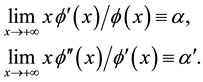
7) If for some fixed there exists a finite limit

(2.7)

then and. For a proof see Agnew ([14] ; Th. 6.2, p. 17).

8) If there exists a finite limit

(2.8)

then and. This has been proved by Agnew ([14] ; Th. 4.2, p. 13) using a non-elementary indirect argument based on the foregoing result and another theorem of his.

9) If it is a trivial fact that relation

(2.9)

does not necessarily imply, the converse inference being true; but relation (2.9) is equivalent to and, if this is the case, then. In fact

(2.10)

The last relation also implies the following version of L’Hospital’s rule for functions in:

Proposition 2.2. If and and then the exists in and equals.

For the proof just write, and apply (2.10). W

10) The space has a link with the classical concept of Cesàro-summability. A function is said to be Cesàro-summable of order one, or summable, on if the following limit

(2.11)

This concept is an extension to improper integrals of the concept of arithmetical mean for a sequence, see Hardy ([15] ; pp. 430-434) and ([16] ; Ch. V and p. 110). It follows from our definition that “f is summable (C, 1) on iff”.

11) Two negative properties concerning functions in.

a) Not any bounded function belongs to. Counterexample:

(2.12)

even if f is uniformly continuous on. In Blinov [17] there is a more elaborate counterexample of a bounded uniformly-continuous function constructed with the implicit use of almost-periodic functions.

For f bounded, the contingency “” can be characterized via the behavior at the origin of the Laplace-transform of f: see either Ditkine and Proudnikov ([18] ; Th. 4, p. 196) or Baumgärtel and Wollenberg ([19] ; Ch. 6, pp. 97-98) where the problem is treated in a functional-analytic context.

b) In general no information on the order of growth of a function in can be drawn. For the function

(2.13)

we have

(2.14)

but;.

All the above properties, from 1 to 9, practically are sufficient conditions for, none of them being characteristic. A counterexample for the converse of property in 6 is provided by:

(2.15)

12) However in Ostrowski ([20] ; IV, pp. 65-68) the following characterization is reported:

The number in Definition 2.1 exists iff

(2.16)

and, if this is the case,.

This result, used by Ostrowski, e.g., in the study of Frullani’s integral, may also yield the nice geometric characterization of a rectilinear asymptote, see (3.15) below. But in other asymptotic investigations a more general form of condition (2.16) is encountered, namely

(2.17)

where stands for some suitable function such that. The number is a kind of “weighted asymptotic mean” of f and can be considered, the sign apart, as a “generalized limit of as” for the simple reason that a trivial application of L’Hospital’s rule yields

under obvious hypotheses on.

The notion of regular variation gives the key to finding out a large meaningful class of test-functions, including powers, such that (2.17), valid for one fixed, is equivalent to.

2.2. Preliminaries on Regularly- or Rapidly-Varying Functions

We use the notion of variation, either regular or rapid, in a restricted sense; for the general theory the reader is referred to the monograph by Bingham, Goldie and Teugels [21] . We get three different results for the three classes defined in

Definition 2.2. Let 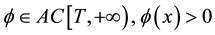for each x large enough.

(I) is termed “regularly varying at +∞ (in the strong sense)” if

(2.18)

for some constant which is called the index of regular variation of at +∞. The family of all such functions for a fixed is denoted by. In the case the function is also termed “slowly varying at +∞ (in the strong sense)”.

(II) is termed “rapidly varying at +∞ (in the strong sense)” if

(2.19)

Accordingly, the index of rapid variation at +∞ is defined to be either +∞ or −∞ and the corresponding families of functions are denoted by and.

(III) is said to have an “index of variation at +∞ in the strong sense” if the following limit exists in the extended real line:

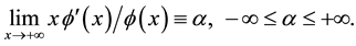(2.20)

Remarks 1) Condition “ultimately of one strict sign” is essential both in the general and in our restricted definition. The choice is merely conventional. Writing tacitly implies “for some T and for x large enough”.

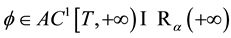
2) Typical functions in, are: where denotes the k-time iterated logarithm, , and,’s are any real numbers.

Typical functions in are:

Here the

index of variation is:.

3) For too has ultimately one strict sign and there are two contingencies for the limit

(2.21)

as inferrred from the identity

For all the possible contingencies may occur for this limit as shown by the functions: 1;,

with;,.

4) If with, it may happen that has no index of variation at +∞ as shown by the counterexamples:

(2.22)

But if has an index of variation then there are precise links between the two indexes.

Lemma 2.3. If and if both and have indexes of variation at +∞, respectively and, then:

(2.23)

In the case and without the stated additional condition on, it may happen that with as shown by the simple examples:

(2.24)

but it cannot be.

2.3. Relationships between Asymptotic Mean and Weighted Asymptotic Means

We can now give and understand generalizations of the mentioned results by Ostrowski and Agnew.

Theorem 2.4. Let and.

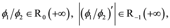
(I) (Regularly-varying functions: extension of a result by Ostrowski, 1976). If

(2.25)

then for any fixed conditions (2.1) and (2.17) are equivalent to each other. If this is the case then, hence does not depend on. An equivalent statement is:

Under conditions (2.25) the following two asymptotic relations are equivalent to each other:

(2.26)

for a constant a which turns out to depend only on f. In one direction we have that the first relation in (2.26), which is trivially true whenever, holds true under the weaker condition.

(II) (Slowly-varying functions). If

(2.27)

then for any fixed condition (2.1) implies (2.17) with.

(III) (Rapidly-varying functions: extension of a result by Agnew, 1942). If

(2.28)1

(2.28)2

(2.28)3

(which imply that both are rapidly-varying at +∞) then for any fixed condition (2.17) implies (2.1) with.

Corollary 2.5. Special cases reformulated:

(2.29)

(2.30)

(2.31)

For the equivalence in (2.29) is Ostrowski’s result, see (2.16), and for the inference in (2.31) is Agnew’s result, see (2.9).

A counterexample for the converse inference in part (II) is provided by:

(2.32)

where the last relation can be easily proved by suitably integrating by parts.

And a counterexample for the converse inference in part (III) is trivially provided by:

(2.33)

Notice that may be rapidly varying without satisfying (2.28)₃ as shown by the function . We do not know if part (III) remains true when replacing the three conditions (2.28) by the weaker conditions:.

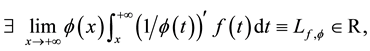
We add the following isolated result, needed in the sequel, without placing it in a general context.

Proposition 2.6. If then:

(2.34)

We end this section by mentioning that the concept of asymptotic mean plays a role also in “Tauberian theorems”, Hardy ([16] ; Ch. 12), in non-oscillation properties of second-order differential equations, Hartman [22] and ([23] ; pp. 365-367), and in the theory of Cauchy-Frullani integrals, Ostrowski [20] . In this last paper our Theorem 2.4-(I) appears for the first time in the literature though for the special case and the proof is somewhat involved. In a previous paper Ostrowski ([13] ; Lemma II) had given a quick proof of a lemma correlated to our present context, a proof based on integration by parts; curiously enough he does not apply the same elementary device in proving the result under consideration, which is just the device used by us to prove the general case. Also the original proof by Agnew [14] is indirect; the author is interested in studying the limit

(2.35)

where is a real number independent from. He first proves the equivalence between (2.8) and (2.35) and then that (2.35) implies.

3. Polynomial Asymptotic Expansions and Asymptotic Means

If, then is defined almost everywhere and for each such t let us consider the “nth-order osculating parabola” to the graph of f at the point:

(3.1)

which may be rewritten in the form

(3.2)

where is a polynomial in x of degree, whose coefficients depend on the parameter t. If all the limits

(3.3)

exist as finite numbers, we say that the parabola

(3.4)

or equivalently the polynomial, is the “nth-order limit parabola” to [the graph of] f at +∞. A limit parabola of order zero denotes a mere relation

We shall call the function the “nth-order contact indicatrix” of the curve with respect to the y-axis as it represents the ordinate of the point of intersection in the x, y-plane between the y-axis and the curve (3.1).

We report here simplified versions of two of the main results in [1] .

Proposition 3.1. For, the following are equivalent properties:

1) The graph of f has a limit parabola at of order n i.e., by definition, all the limits

(3.5)

2) The single limit

(3.6)

3) There exists a polynomial such that

(3.7)

If this is the case then the following integral representation holds true

(3.8)

for a suitable polynomial, the same as above, and a suitable number, the same as in (3.6).

We expressed relations in (3.7) by saying that the asymptotic expansion

(3.9)

is formally differentiable n times in the “strong sense” because in the same paper we characterized another weaker set of differentiated expansions, ([1] ; Th. 3.1, p. 173), which we shall not presently use.

Proposition 3.2. If and is convex of order on―which is equivalent to the property that is increasing thereon―then: f has a “polynomial asymptotic expansion at +∞”, i.e. it satisfies a relation of type

(3.10)

iff its nth-order contact indicatrix is bounded (hence, by monotonicity, condition (3.6) holds true). If this is the case then we also have the properties in Proposition 3.1, hence the expansion (3.10) automatically implies its formal differentiability n times in the strong sense.

Now we give analogues of the two foregoing propositions with condition (3.6) replaced by the weaker condition; strong differentiability will be granted times and the validity of an expansion (3.10) will be characterized for a class of functions larger than nth-order convexity.

Theorem 3.3. For, the following are equivalent properties:

1) All the functions

(3.11)

2) The single function

(3.12)

3) There exists a polynomial such that

(3.13)

If this is the case then and the following integral representation holds true:

(3.14)

In the elementary case n = 1 the result is:

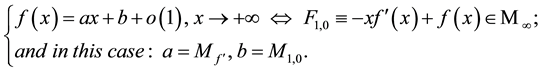(3.15)

Notice that the representation of inferred from (3.14) contains the quantity hence, by the example in (2.13), no information on the growth-order of may be obtained in the context of Theorem 3.3, generally speaking.

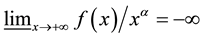
For a characterization similar to that in (3.15) holds true under a restriction on the sign of and we have the following analogue of Proposition 3.2.

Theorem 3.4. Let and let satisfy a one-sided boundedness condition:

(3.16)

Then an expansion (3.10) holds true iff. If this is the case then, according to Theorem 3.3, the expansion (3.10) is formally differentiable times in the strong sense.

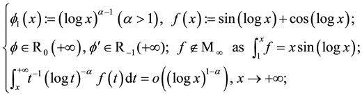
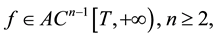
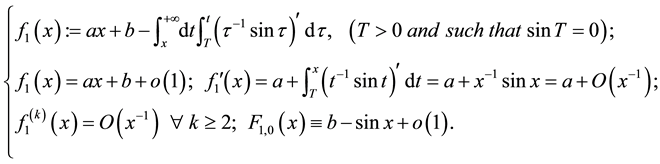
We exhibit an example for the case and a counterexample for the case; they seem to be just the same because in both expansions the remainder is exactly the same quantity but a striking difference appears in the behaviors of and.

Example for the case:

(3.17)

Here is bounded and admits of asymptotic mean but has no limit at +∞; accordingly the expansion is not formally differentiable in the strong sense though the differentiated expansions of any order satisfy the remarkable asymptotic estimates in (3.17).

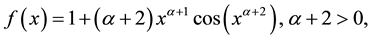
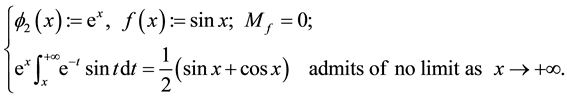
Counterexample for the case:

(3.18)

Here is unbounded both from below and from above and admits of no asymptotic mean; notwithstanding, an asymptotic expansion holds true. Hence the equivalence stated in Theorem 3.4 may fail without the restriction in (3.16). According to Theorem 3.3 the expansion of f₂ is not formally differentiable once in the strong sense.

In the elementary case in (3.15) condition is explicitly defined in Giblin ([24] ; p. 279) as the “bounded distance condition” and it is easily checked that it is equivalent to a pair of relations

(3.19)

it is the further condition of existence of asymptotic mean that changes the first relation in (3.19) into an asymptotic straight line.

4. Two-Term Asymptotic Expansions and Asymptotic Means

In this section we give an exhaustive list of results concerning the role of asymptotic mean in the theory of two-term asymptotic expansions involving comparison functions admitting of indexes of variation at +∞. We first report a result from [4] .

Preliminary notations and formulas ([4] ; p. 255). As usual we say that two functions f, g (as well as their graphs) have a first-order contact at a point t₀ if and provided that f, g are defined on a neighborhood of t₀ and the involved derivatives exist as finite numbers.

Let now, be two real-valued functions differentiable on an interval I such that their Wronskian never vanishes on I and let f be differentiable on I. Then for each there exists a unique function in the family having a first-order contact with f at t₀. Denoting this function by we have

(4.1)

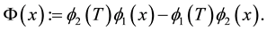
where

(4.2)

If then on I for any chosen t₀. The function

(4.3)

will be called the contact indicatrix of order one of the function f at the point t with respect to the family and the straight line.

represents the ordinate of the point of intersection between the vertical line and the curve where t is thought of as fixed. The assumption on implies that and do not vanish simultaneously hence is a nontrivial linear combination of,. It may happen that, for some choices of T, coincides with or, a constant factor apart, according as or.

Using (4.2) may be represented as

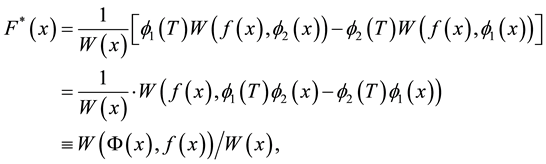(4.4)

where we have put

(4.5)

Proposition 4.1. (Characterization of a two-term asymptotic expansion: [4] , Th. 4.4, p. 258). Assumptions:

(4.6)

(4.7)

For a function the following are equivalent properties:

1) It holds true an asymptotic expansion

(4.8)

2) There exists a finite limit

(4.9)

3) There exists a finite limit

(4.10)

If this is the case we have the following two representations:

(4.11)

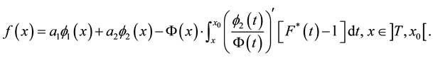(4.12)

The validity of (4.8) may be expressed by the geometric locution: “the graph of f admits of the curve as an asymptotic curve in the family, as.”

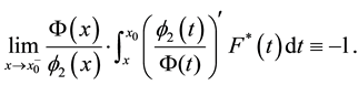
Notice that in the cited reference condition (4.10) is written in the form

(4.13)

however (4.5) implies

(4.14)

and (4.10) follows.

The two limits in (4.9), (4.10) are of the type studied in §2 and a direct application of Theorem 2.4 gives the following results.

Theorem 4.2. In assumptions (4.6)-(4.7) let it be:;.

(I) (Regularly-varying comparison functions). If

(4.15)

then the following three properties are equivalent:

(4.16)

(4.17)

(4.18)

(II) (Slowly-varying comparison functions). If

(4.19)

then each condition (4.17) or (4.18) implies an expansion (4.16).

(III) (Rapidly-varying comparison functions). Put and suppose that:

(4.20)

then an expansion (4.16) implies both conditions (4.17)-(4.18).

Under the stated assumptions for the validity of part (I) the equivalence “(4.16) Û (4.18)” admits of the following geometric reformulation:

“The graph of f admits of an asymptotic curve in the family, as, iff the contact indicatrix of order one of the function f with respect to has an asymptotic mean at +∞”.

Notice that this result for two-term expansions requires no restrictions on the signs of,.

5. Proofs

Proof of Lemma 2.3. By hypothesis the following two limits exist in:

(5.1)

We now evaluate by L’Hospital’s rule first noticing that: implies, whereas for it is and the first limit in (5.1) implies. In both cases the rule may be applied and

(5.2)

It remains the case which implies and this condition leads to excluding the following contingencies for the indicated reasons:

1)

2) (by L’Hospital’s rule)

which is a positive real number; hence which would imply.

3) and this would imply, by L’Hospital’s rule as in (5.2):.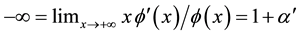

4) The case must be treated in a different way. A basic property of our class of functions, directly inferred from the limits in (5.1), claims the validity of the following asymptotic estimates:

(5.3)

Now in our present proof we have and, hence

and there are two a-priori contingencies about the integral. Its divergence would imply which cannot be; in the other case we would have

(5.4)

which contradicts the second relation in (5.3). Notice that the procedure used to prove this last case works for any as well.

The last assertion in the statement of Lemma 2.3, namely “it cannot be”, follows from the calculations in 2): implies, but in this case (5.2) shows, a contradiction. W

Proof of Theorem 2.4. (I) We make explicit the assumptions writing:

(5.5)

which in turn imply the following relations to be used in the sequel:

(5.6)

(5.7)

(5.8)

First part: (2.17) Þ (2.1). If we put

(5.9)

then, by (2.17), we may write

(5.10)

From (5.9) and (2.17):

(5.11)

(5.12)

(5.13)

Using (5.11) and (5.13) in the left side of (5.10) we get, i.e. (2.1).

Second part: (2.1) Þ (2.17). First step: convergence of Consider the identity

(5.14)

and estimate the behavior of as. From (2.1) and 5.8) we get:

(5.15)

(5.16)

As concerns we have:

(5.17)

from whence and (2.1) we get:

(5.18)

As, we obtain the convergence of hence, by (5.14), of.

Second step: asymptotic behavior of. By (5.16) and (5.18) we may integrate by parts as follows:

(5.19)

which is (2.17) with.

(II) From the first assumption in (2.27) we infer:

(5.20)

and from (5.17):

(5.21)

Now we retrace all steps in the second part of the proof of part (I) checking the validity of the corresponding formulas for. Instead of the first relation in (5.16) we have:

(5.22)

and, instead of (5.18):

(5.23)

The convergence of follows as above. And using the same integration by parts as in (5.19) we get the same final relation.

(III) Let us first show that the three conditions in (2.28) imply that both are rapidly-varying at +∞. Conditions in (2.28)_1,2 are equivalent to, and (2.28)₃ is equivalent to

(5.24)

which implies, by (2.28)₁, ultimately; so we have:

Now we retrace all steps in the first part of the proof of part (I) and again use decomposition (5.10); instead of (5.11) we get:

(5.25)

and instead of (5.12) we get, using (5.24):

(5.26)

whence

(5.27)

From (5.25), (5.26), (5.27) we get (2.1) with. W

Proof of Proposition 2.6. Integration by parts gives:

(5.28)

whence our claim follows dividing both sides by x. W

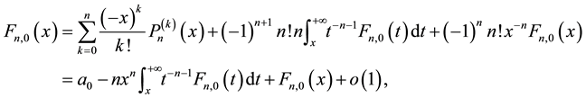
Proof of Theorem 3.3. Let us assume (3.12) and start from the integral representation ([1] ; formula (6.3), p. 185):

(5.29)

which for reads:

(5.30)

From (5.30) the elementary equivalence in (3.14) easily follows, hence we suppose. If (3.12) holds true and we apply the asymptotic relation in (2.29) to we get:

(5.31)

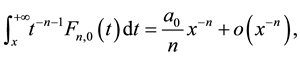
and the last relation, when replaced into (5.29), yields:

(5.32)

But the first relation in (5.31) implies that the iterated improper integral converges and we get a representation of type:

(5.33)

together with the expansion:

(5.34)

having used one of the following elementary identities (to be used again):

(5.35)

To prove the formal differentiabilty we put:

(5.36)

and from (5.31) we infer relations:

(5.37)

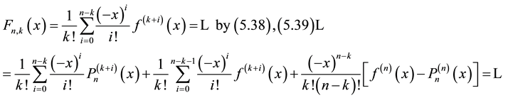
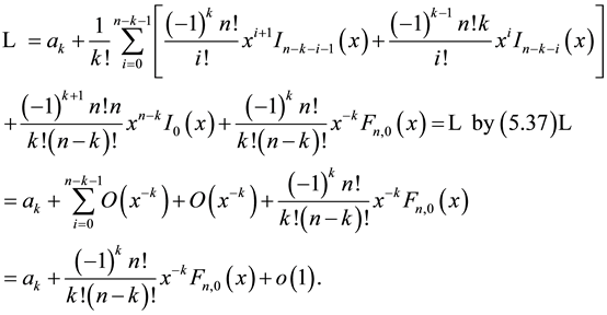
Calling the last sum on the right in (5.34), which differ by a constant from the sum on the right in (5.33), and applying Leibniz's rule to (5.33) we get:

(5.38)

The expressions of and involve and its derivative:

(5.39)

So far we have proved that (3.12) implies relations in (3.13) for, without any information on, and, for the time being, is a non-better specified polynomial of degree. To prove (3.11) we estimate the behavior, as, of for using its known expression in terms of f, ([1] ; formula (2.6), p. 168):

(5.40)

as the first sum is nothing but the expression of the coefficient of the power in the polynomial, i.e.,

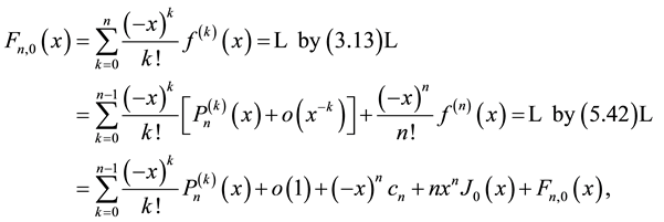
By (2.34) the function has asymptotic mean “zero” and the same is true for a term; so the sum of the last three terms above represents a function with asymptotic mean equalling. We have proved that “2) Þ 1) Ù 3)”. It remains to show “3) Þ 2)”. First step. Let us first evaluate from representation (5.29); putting

(5.41)

we get:

(5.42)

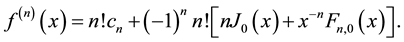
Now we start as in (5.40) from the expression of:

(5.43)

whence we get

(5.44)

which implies the convergence of the improper integral; and we can rewrite representation (5.29) in the form:

(5.45)

Comparing (5.45) and the assumed relation we infer that the two polynomials and the sum appearing in (5.45) have the same leading coefficient:. Now we do calculations just like those from (5.41) to (5.43) but starting from representation (5.45) and paying attention to the signs, so getting:

(5.46)

(5.47)

having used the identity, ([1] ; Lemma 2.2, p. 169). From (5.47) we infer

(5.48)

which, by (2.29), implies and. W

Proof of Theorem 3.4. The only thing to be proved is that an expansion (3.10) plus condition (3.16) imply. We first show that it is enough to prove our claim with (3.16) replaced by the condition of one-signedness:

(5.49)

In fact it is known, ([1] ; Lemma 2.2, p. 169), that: iff f is a polynomial of type

(5.50)

Let now g be any function, , let p be a polynomial of type (5.50) and define: . With an obvious meaning of the symbol we have:; hence:

(5.51)

It follows that any result on formal differentiability of a polynomial asymptotic expansion involving g admits of a literal transposition to a polynomial asymptotic expansion involving f. Our assumption are now: expansion (3.10) and one-signedness of, and the proof (which we make explicit here) is a word-for-word repetition of that in ([1] ; Proof of Th. 4.2, pp. 193-195) with a slight modification at the conclusive passage. From representation (5.29) we infer

(5.52)

and, by (3.10), the following limit:

(5.53)

For (3.10) reduces to and (5.53) is “convergent”. Hence representation (5.29) can be rewritten in the form

and (3.10) implies that “exists in” which is equivalent to.

For we apply L’Hospital’s rule times to the limit in (5.53) so getting the limit:

(5.54)

By the one-signedness of this last limit exists in the extended real line, hence it must be a finite number. This means the convergence of and representation (5.29) can be rewritten as:

(5.55)

The last relation implies that coincides with the in (3.10) and we get:

(5.56)

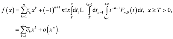
By the above argument involving L’Hospital’s rule we arrive at the convergence of the iterated integral

. An iteration of the procedure yields condition

(5.57)

which implies representation

(5.58)

where the coefficients are those in (3.10). From (5.58) we infer that

(5.59)

and applications of L’Hospital’s rule times yields the limit

(5.60)

which, by (2.29), is equivalent to. W

In passing notice that the last calculations and (5.34) prove that:

For a given function and g one-signed the following equivalence holds true:

(5.61)

References

- Granata, A. (2007) Polynomial Asymptotic Expansions in the Real Domain: The Geometric, the Factorizational, and the Stabilization Approaches. Analysis Mathematica, 33, 161-198. http://dx.doi.org/10.1007/s10476-007-0301-0
- Granata, A. (2010) The Problem of Differentiating an Asymptotic Expansion in Real Powers. Part I: Unsatisfactory or Partial Results by Classical Approaches. Analysis Mathematica, 36, 85-112. http://dx.doi.org/10.1007/s10476-010-0201-6
- Granata, A. (2010) The Problem of Differentiating an Asymptotic Expansion in Real Powers. Part II: Factorizational Theory. Analysis Mathematica, 36, 173-218. http://dx.doi.org/10.1007/s10476-010-0301-3
- Granata, A. (2011) Analytic Theory of Finite Asymptotic Expansions in the Real Domain. Part I: Two-Term Expansions of Differentiable Functions. Analysis Mathematica, 37, 245-287. (For an Enlarged Version with Corrected Misprints see: arxiv.org/abs/1405.6745v1 [mathCA]. http://dx.doi.org/10.1007/s10476-011-0402-7
- Granata, A. (2014) Analytic Theory of Finite Asymptotic Expansions in the Real Domain. Part II: The Factorizational Theory for Chebyshev Asymptotic Scales. Electronically Archived―arXiv: 1406.4321v2 [math.CA].
- Granata, A. (2015) The Factorizational Theory of Finite Asymptotic Expansions in the Real Domain: A Survey of the Main Results. Advances in Pure Mathematics, 5, 1-20. http://dx.doi.org/10.4236/apm.2015.51001
- Haupt, O. (1922) Über Asymptoten ebener Kurven. Journal für die Reine und Angewandte Mathematik, 152, 6-10; ibidem, 239.
- Sanders, J.A. and Verhulst, F. (1985) Averaging Methods in Nonlinear Dynamical Systems. Springer-Verlag, New York.
- Corduneanu, C. (1968) Almost Periodic Functions. Interscience Publishers, New York.
- Faedo, S. (1946) Il Teorema di Fuchs per le Equazioni Differenziali Lineari a Coefficienti non Analitici e Proprietà Asintotiche delle Soluzioni. Annali di Matematica Pura ed Applicata (the 4th Series), 25, 111-133. http://dx.doi.org/10.1007/BF02418080
- Hallam, T.G. (1967) Asymptotic Behavior of the Solutions of a Nonhomogeneous Singular Equation. Journal of Differential Equations, 3, 135-152. http://dx.doi.org/10.1016/0022-0396(67)90011-3
- Hukuhara, M. (1934) Sur les Points Singuliers des Équations Différentielles Linéaires; Domaine Réel. Journal of the Faculty of Science, Hokkaido University, Ser. I, 2, 13-88.
- Ostrowski, A.M. (1951) Note on an Infinite Integral. Duke Mathematical Journal, 18, 355-359. http://dx.doi.org/10.1215/S0012-7094-51-01826-1
- Agnew, R.P. (1942) Limits of Integrals. Duke Mathematical Journal, 9, 10-19. http://dx.doi.org/10.1215/S0012-7094-42-00902-5
- Hardy, G.H. (1911) Fourier’s Double Integral and the Theory of Divergent Integrals. Transactions of the Cambridge Philosophical Society, 21, 427-451.
- Hardy, G.H. (1949) Divergent Series. Oxford University Press, Oxford. (Reprinted in 1973)
- Blinov, I.N. (1983) Absence of Exact Mean Values for Certain Bounded Functions. Izvestija Akademii Nauk SSSR. Serija Mathematicheskaja (Moscow), 47, 1162-1181.
- Ditkine, V. and Proudnikov, A. (1979) Calcul Opérationnel. Éditions Mir, Moscou.
- Baumgärtel, H. and Wollenberg, M. (1983) Mathematical Scattering Theory. Birkhäuser Verlag, Berlin.
- Ostrowski, A.M. (1976) On Cauchy-Frullani Integrals. Commentarii Mathematici Helvetici, 51, 57-91. http://dx.doi.org/10.1007/BF02568143
- Bingham, N.H., Goldie, C.M. and Teugels, J.L. (1987) Regular Variation. Cambridge University Press, Cambridge. http://dx.doi.org/10.1017/CBO9780511721434
- Hartman, Ph. (1952) On Non-Oscillatory Linear Differential Equations of Second Order. American Journal of Mathematics, 74, 389-400. http://dx.doi.org/10.2307/2372004
- Hartman, Ph. (1982) Ordinary Differential Equations. 2nd Edition, Birkhäuser, Boston.
- Giblin, P.J. (1972) What Is an Asymptote? The Mathematical Gazette, 56, 274-284. http://dx.doi.org/10.2307/3617830