Atmospheric and Climate Sciences
Vol.06 No.03(2016), Article ID:68368,30 pages
10.4236/acs.2016.63036
Assessment of Climate Change in Nicaragua: Analysis of Precipitation and Temperature by Dynamical Downscaling over a 30-Year Horizon
Josep Maria Solé1, Raúl Arasa1, Miquel Picanyol1, Mª Ángeles González1, Anna Domingo-Dalmau1, Marta Masdeu1, Ignasi Porras1, Bernat Codina1,2
1Technical Department, Meteosim S.L., Barcelona, Spain
2Department of Astronomy and Meteorology, University of Barcelona, Barcelona, Spain

Copyright © 2016 by authors and Scientific Research Publishing Inc.
This work is licensed under the Creative Commons Attribution International License (CC BY).
http://creativecommons.org/licenses/by/4.0/


Received 3 June 2016; accepted 11 July 2016; published 14 July 2016
ABSTRACT
The present study has generated and analyzed Climate Change projections in Nicaragua for the period 2010-2040. The obtained results are to be used for evaluating and planning more resilient transport infrastructures in the next decades. This study has focused its efforts to pay attention into the effect of Climate Change on precipitation and temperature from a mean and extreme event perspective. Dynamical Downscaling approach on a 4 km resolution grid has been chosen as the most appropriate methodology for the estimation of the projected climate, being able to account for local-scale factors like complex topography or local land uses properly. We selected MPI- ESM-MR as the global climate model with the best skill scores in terms of precipitation and temperature in Nicaragua. MPI-ESM-MR was coupled to a mesoscale model. We chose WRF mesoescale model as the most appropriate regional model and we optimized their physical and dynamical options in order to minimize the model uncertainty in Nicaragua. For this, model output against the available in-situ measurements from the national meteorological station network and satellite data were compared. Climate change signal was estimated by comparing the different climate statistics calculated from a model run over an historical period, 1980-2009, with a model run over a projected period, 2010-2040. The obtained results from the projected climate show an increase of the mean temperature between 0.6˚C and 0.8˚C and an increase of the number of days per year with maximum daily temperatures higher than 35˚C. Regarding precipitation, annual projected amounts do not change remarkably with respect to the historical period. However, significant changes in the distribution of the precipitation within the wet period (May-October) were observed. Moreover, an increment between 5% and 10% of the number of days without precipitation is expected. Finally, Intensity-Duration-Frequency (IDF) projected curves show an increment of the rainfall intensity and an increment of extreme precipitation event frequency, especially in the Caribbean basin.
Keywords:
WRF, Climate Change, Global Warming, Dynamical Downscaling, Precipitation Projections, IDF

1. Introduction
Climate change is one of the main challenges of modern society. The impact of climate change is global and delocalized of anthropogenic emissions that induce it and, for this reason, it is essential to achieve global agreements to combat it. Global warming and climate change are mainly caused by emissions of greenhouse gases and aerosols emitted by industry, mainly traffic and residential heating [1] . For years, nations around the world have tried to achieve compromises to reduce these emissions and they have organized meetings and conventions to reach binding agreements. And in the last annual conference of parties (COP), 195 countries adopted the first universal climate agreement (United Nations Conference on Climate Change in Paris, COP’21, http://www.cop21.gouv.fr/en).
Climate change affects meteorology and climate, modifying the Earth radiation balance, and consequently, affecting meteorological variables as temperature and precipitation, weather patterns like El Niño, and altering the natural frequency of extreme events as hurricanes and tropical cyclones. But their impacts cover all aspects of the society, affecting transports, infrastructures, agriculture, economy, ecosystems, vegetation, land uses and regional planning, migrations, etc.
Nicaragua is particularly vulnerable to the effects of Climate Change due to its location in the inter-tropical convergence zone, being one of the economies most exposed to climate hazards. The highest risk area is the northern Caribbean coast, gradually decreasing towards to south, and floods and landslides are recurrent in the country. In the recent history, these impacts have produced direct and indirect economical losses. It was estimated that annual economic losses due to extreme weather events (e.g. hurricanes, tropical storms, floods and landslides, excluding droughts) between 1990 and 2012 were 1.89% of GDP [2] . For example, hurricane Félix (2007) caused damage equivalent to 14.4% of GDP, while extreme and heavy precipitations that affected the northwest of the country in 2011 and 2012 caused damages equal to 3% and 6.8% of GDP respectively according to data from World Bank. Hurricane Mitch (1998) is considered to date as the most serious climate disaster in the recent history of Central America, affecting 90% of the territory and causing 3800 fatalities in Nicaragua, and numerous people are displaced. In contrast to this, a part of the territory of Nicaragua is also prone to severe drought, especially along the “dry corridor” of Central America that affects 20% of the territory of Nicaragua. For all these reasons, Nicaragua is a highly vulnerable region to its current climate, and climate change effects can even increase the existent hazards or cause new ones. Trying to reduce the impact of these events, the Government of Nicaragua and other multilateral institutions as the Nordic Development Fund or the World Bank have promoted different studies with the aim to increase the adaptability of the country to the effects of Climate Change [3] - [6] .
Climate research centers have addressed the climate change analysis by global modeling, projecting the future climate under various scenarios of anthropogenic emissions. Due to computational limitations, the usual resolution of global climate models is very low and, therefore, only allows reproducing synoptic scale phenomena. Consequently, and due to the geographical features of Nicaragua and its topographic complexity, the results of the global climate models cannot be used for the evaluation of the local effects of climate change over Nicaragua. To address this problem it is necessary to apply techniques of downscaling that allow increasing the resolution of the results obtained through global climate models [7] [8] . There are two kinds of downscaling: statistical and dynamical regionalization. The first one corresponds to a mathematical or statistical approach, based on the definition of statistical patterns using historical weather information from measurement data [9] - [11] , and dynamical downscaling which corresponds to a physical approach, based on the equations governing the behavior of the atmosphere [11] - [14] . Dynamical downscaling is a technique more expensive than statistical downscaling from the point of view of computational cost.
The study we present here is innovative for two reasons: 1) it is the first time that the technique of dynamical downscaling using a mesoscale meteorological model is applied over Nicaragua, and few studies of dynamical downscaling have been realized in Central America; and 2) the study uses and configures, for the first time in Nicaragua, a mesoscale meteorological model, increasing extensively the horizontal resolution used in the previous studies in the country, obtaining the local effect of climate change for all of Nicaragua in a 4 km horizontal grid.
Description of the climate features of Nicaragua and their climatic regions is presented in section 2. In section 3 a complete description of the dynamical downscaling methodology defined and developed is shown. An analysis of the results obtained is presented in section 4 and, finally, conclusions are reported in section 5.
2. Geographic Information, Climate Features and Climate Regions of Nicaragua
Nicaragua is located in Central America in tropical latitudes between 10˚N and 15˚N. It borders both by Caribbean Sea and North Pacific in east and west boundaries respectively and by Costa Rica and Honduras in south and north boundaries respectively. Nicaragua is divided into 17 departments and Managua is the capital city (Figure 1).
Nicaragua extends an area about 130,000 km2 containing a wide range of climates and land uses. Nicaraguan topography is complex consisting of a Central Highlands which divides the country into the Pacific and Caribbean lowlands. The Pacific lowland consists of a flat area with a volcanic chain and two freshwater lakes: Cocibolca and Xolotlán with an extension about 8200 and 1000 km2. Central Highlands comprise a triangular area with ridges from 900 to 1800 m.a.s.l composed by “Cordillera Isabelia” y “Cordillera Amerrisque” (Figure 1). The Caribbean lowland is sparsely settled and includes coastal plains and the lower area of Río San Juan.
Nicaragua. Main geographical features of the country are: Cocibolca and Xolotlán lakes (also called Nicaragua and Managua lakes respectively), connected by the Tipitapa River; Mogoton is the highest mountain in Nicaragua, reaching 2107 m.a.s.l, located in the Cordillera Isabelia in the northern portion of the central mountain range, which runs from northwest to southeast through the center of the country; and main rivers are the San Juan, Coco, Grande and Escondido.
Climate features in Nicaragua are driven by multiple factors which can act simultaneously and are related each other. The proximity to the Pacific Ocean and the Caribbean Sea, its tropical location and its complex topography

 (a) (b)
Figure 1. Geographical features and location of meteorological stations from INETER network with precipitation measurements and temperature measurements (a). NP represents North Pacific; CP―Central Pacific; SP―South Pacific; NZ―North Zone; CZ―Central Zone; NC―North Caribbean; SC―South Caribbean. And territorial division of Nicaragua (b).
result in a complex meteorological system highly variable in time and space.
Due to its tropical latitudes, Nicaragua is within the Intertropical Convergence Zone (ITCZ) depending on the season. Therefore, this region (in the Northern Hemisphere) is typically influenced by Northeast trade winds and an important convection activity.
Due to the influence of the Caribbean Sea, Nicaragua is periodically affected by hurricanes and tropical cyclones normally occurring from May to October. At the same time, Nicaragua is located under the influence of the Pacific Ocean which configures a rainfall regime based on two seasons: a wet season from May to October and a dry season from November to April. Due to its proximity to the Pacific Ocean, Nicaragua is under the effect of ENSO (El Niño-Southern Oscillation) which can alter the rainfall regime oceanic year-to-year. A positive-El Niño-(or a negative-La Niña) anomaly of Sea Surface Temperature in the Easter Equatorial Pacific Ocean (defined as Niño 3.4 region) is normally correlated with a strong (or a weak) dry period in the Pacific Basin and, at the same time, is correlated with an increase(or decrease) of Caribbean hurricanes frequency in the Caribbean Basin respectively.
Indeed, Nicaragua has a very complex topography with volcanic structures and abrupt mountain ranges which divide the country in 7 climate regions which are defined by INETER (Nicaraguan Institute of Territorial Studies) and shown in Figure 1. The main singularities of each in terms of temperature and precipitation are described below based on temperature and precipitation monthly-mean data of INETER meteorological network. As can be seen in Figure 1, temperature and precipitation meteorological stations are not distributed spatially uniformly, but also they are denser in the Pacific regions than in the Caribbean regions.
・ North Pacific (NP): It is located on the northwestern sector with presence of several volcanic cones and low topography complexity. Temperature annual profile is based on monthly mean temperatures above 26˚C throughout the year with maximum temperatures in April reaching monthly means above 28˚C. Precipitation is based on a two-season profile with a dry season from December to April and a wet season from May to November. Within the wet season a double peak is observed with a first precipitation maximum in May- June and a second one in October. Annual precipitation is normally between 1000 and 2000 mm.
・ Central Pacific (CP): It is located on the central western sector with presence of several volcanic cones and low topography complexity. Temperature annual profile and precipitation profile is very similar to North Pacific profile, although the presence of Cocibolca and Xolotlán lakes implies a slight softening of precipitation and temperature profiles in comparison with North Pacific. Annual precipitation is normally between 1000 and 2000 mm.
・ South Pacific (SP): It is located on the southwestern sector with presence of several volcanic cones and low topography complexity. Temperature annual profile and precipitation profile is very similar to North Pacific and Central Pacific profile. The presence of Cocibolca and Xolotlán clearly affect to the precipitation profile with a double-peak less noticeable in the wet period. Annual precipitation is normally between 1000 and 2000 mm.
・ North Zone (NZ): It is located on the northern sector with presence of the highest and the most abrupt mountain ranges with a high topography complexity. Temperature annual profile shows mean temperatures above 22 degrees throughout the year with maximum temperatures in April-May. Precipitation profile shows a two-season profile as shown in Pacific regions with a strong dry period from December to April and a weak wet period from May to November. Annual precipitation is normally below 1000 mm.
・ Central Zone (CZ): It is located on the southern sector with presence of the high mountain range like Amerrisque. Temperature annual profile shows temperatures above 25 degrees throughout the year with maximum temperatures in April-May. Precipitation profile shows a two-season profile as shown in Pacific regions with a strong dry period from December to April and a wet period from May to November. The double-peak in the wet period is less noticeable due to the influence of lakes. Annual precipitation is normally between 1000 and 2000 mm.
・ North Caribbean (NC) and South Caribbean (SC): It is located on the northeastern and southeastern sector respectively. Its temperature annual profile shows soft temperatures above 24 degrees with maximum temperatures in April-May. Precipitation is present throughout the year, although a substantial decrease occurs between December and April. Annual precipitation is normally between 2000 and 4000 mm.
3. Methodology: Dynamical Downscaling
Dynamical downscaling for climate applications is defined as a technique based on coupling a global climate model (GCM) and a regional climate model (RCM) [15] . The regional model is running over a limited area and is forced by initial and boundary conditions from the global climate model.
In order to implement this methodology we have followed different steps described below in a brief summary and extended it in the next subsections.
1) Selection of the global climate model (GCM) reproducing the best possible the atmospheric conditions of Nicaragua.
2) Analysis and selection of the most convenient Representative Concentration Pathway (RCP) defined as different radiative forcing sin relation to different levels of global warming.
3) Selection and configuration of the regional climate model in order to reduce the uncertainty and increase the accuracy as much as possible in Nicaragua.
4) Validation of the obtained regional climate model configuration through a historical climatic run of 30 years long forced by reanalysis.
5) Design of the regional climate simulations in terms of time segmentation and decision about the historical and the projected time periods.
6) Execution of modeling regional climate runs with the regional model forced by the selected GCM in step (1).
7) Climate change signal estimation by comparing historical and projected runs.
3.1. Global Climate Model
The selection of the most appropriated GCM has involved three different data platforms: Earth System Grid Generation (ESGF) Peer-to-peer enterprise system, CERA WW3-Gateway and CISL Research Data Archive. In these databases numerous and multiple GCM are available. We selected the most convenient according to the following criteria: 1) GCM must be included in the 5th Coupled Model Intercomparison Project (CMIP5); 2) simultaneous availability of historical and projected GCM runs; 3) simultaneous availability of 6-hourly data of temperature, geopotential height, specific humidity, wind velocity and wind direction. As a result, 13 GCM are considered (Table 1).
The selected GCM runs have been validated with temperature and precipitation data from satellite and reanalysis. The validation has been performed in terms of spatial means on Nicaragua delimited by 10 - 15˚N/91 - 96˚W. We used the following databases:
・ Delaware (satellite). To evaluate the temperature over land. Period evaluated: 1980-2009 (http://www.esrl.noaa.gov/psd/data/gridded/data.UDEL_AirT_Precip.html).

Table 1. GCM considered evaluating their accuracy over Nicaragua.
・ GPCC (satellite). To evaluate precipitation over land. Period evaluated: 1980-2009 (ftp://ftp.dwd.de/pub/data/gpcc/html/fulldata_v6_doi_download.html).
We have evaluated the differences between modeled and observed values using root mean square error (RMSE) and Pearson correlation coefficient (r) for: monthly average precipitation and monthly average temperature at 2 meters (Table 2). Results show that MPI-ESM-MR is the GCM that reproduces in the most appropriated way the atmospheric conditions of Nicaragua in terms of precipitation and temperature. The obtained results are consistent with those obtained by Hidalgo and Alfaro [16] . In this study, MPI-ESM-MR is identified as one of the best playing conditions for Central America. Results are complemented with the monthly evolution of temperature and monthly precipitation for every GCM and satellite data (Figure 2).
Radiative scenario
Global Climate models use different climate scenarios based on future projections of radiative forcing associated to different levels of global warming. These scenarios are known as Representative Concentration Pathways (RCPs). The Intergovernmental Panel on Climate Change (IPCC) defines up to 4 RCPs scenarios, identified as RCP2.6, RCP4.5, RCP6.0 and RCP8.5, corresponding to the radiative forcings for the year 2100 of 2.6 W/m2 [17] , 4.5 W/m2 [18] , 6.0 W/m2 [19] [20] and 8.5 W/m2 [21] , respectively. High radiative forcing implies less mitigation measures and higher temperatures, whereas, a less radiative forcing implies more mitigation measures and lower temperatures. Moreover the highest radiative forcing scenario (RCP8.0) corresponds to the worst scenario from the point of view of emissions and, therefore, from the point of view of temperature, but not from the point of view of precipitation, because the relationship is not direct for this variable.
It is impossible to define a scenario as more or less likely than the other, as this will depend on the current and future evolution of greenhouse gases (GHG) emissions, as well as the evolution of many socioeconomic and geopolitical variables. However, for the next thirty years, the application of one or another should not be a factor involving drastic differences in the corresponding climate regional simulations, being 2.999 W/m2, 3.411 W/m2, 3.146 W/m2 and 3.993 W/m2 the radiative forcing projected in the year 2040 for the scenarios RCP2.6, RCP4.5, RCP6.0 and RCP8.5, respectively. For this reason, and because mitigation measures of GHG emissions and strategies and technologies for emissions reduction are already being implemented, the RCP4.5 has been the radiative scenario selected to conduct the dynamical downscaling.
3.2. Regional Model
The regional and mesoscale meteorological model used for the study has been the Weather Research and
Table 2. Correlation coefficient (r) and RMSE calculated using monthly average temperature and accumulated precipitation diagnosed by GCMs and information from satellite and/or reanalysis. Bold mark the optimal values for global model and shaded in blue values corresponding to the MPI-ESM-MR model.


Figure 2. Monthly average temperature (top) and monthly average accumulated precipitation (bottom) diagnosed by the different GCMs evaluated and satellite data.
Forecasting-Advanced Research (WRF-ARW) version 3.7 [22] , developed by the National Center of Atmospheric Research (NCAR). It is a universally used community mesoscale model and a state-of-the-art atmospheric modeling system that is applicable for meteorological research, climate scenarios and numerical weather prediction. WRF is a fully compressible and non-hydrostatic model with terrain-following hydrostatic pressure coordinate. In the next sections, we show the WRF domain, the experiments realized to obtain the best configuration of WRF for Nicaragua and the design of the climate simulations.
Simulation domains and resolution
In Figure 3, we show modeling domains used for simulations. The WRF model is built over a mother domain (d01) with 108 km spatial resolution, centered at 12.15˚N, 86.27˚W, and with a domain size of 9396 × 6588 km2. It comprises Central America, northern South America and southern North America. The first nested domain (d02), with a spatial resolution of 36 km and with a domain size of 5112 × 4140 km2, covers the Atlantic and Pacific region of Central America. The third domain (d03), with a spatial resolution of 12 km and with a domain
d01, d02, d03 and d04
 d04
d04
Figure 3. Modeling domains for simulations.
size of 1776 × 1416 km2, covers Nicaragua, Costa Rica, Panamá, Honduras, El Salvador, Guatemala and Jamaica. And finally, the fourth domain (d04) covers fully Nicaragua with a spatial resolution of 4 km and with a domain size of 688 × 640 km2.
The number of vertical levels used is 30. These vertical layers cover the whole troposphere with a resolution decreasing slowly with height in order to capture low-level flow details.
Sensitive analysis and calibration
Different options that WRF offers can be combined in many different ways. WRF has different parameterizations for microphysics, radiation (long and short wave), cumulus, surface layer, planetary boundary layer (PBL) and land surface as physical options. To obtain WRF highest accuracy, it is essential to carry out a sensitive analysis of these different options by numerical experiments. In the same way, the definition of the simulation domains, spin up, vertical resolution or nesting architecture determine the accuracy, and therefore uncertainty, of WRF results [23] [24] . In this sense, and with the aim to obtain the best WRF configuration for climate applications in Nicaragua, numerical experiments corresponding to different physical and dynamical options have been tested.
There are multiple and numerous combinations of WRF options, being not feasible to analyze all of them. For this reason, and as the goal is to analyze the variables precipitation and temperature, we focus our attention on the study of cumulus, planetary boundary layer parameterization and surface layer scheme options. And we have fixed the rest of options following the NCAR recommendations for regional climate runs. In this way we have used WSM6 [25] , Noah LSM [26] and CAM [27] as microphysical, land surface scheme and radiation options respectively.
A total of 17 experiments have been evaluated progressively, as Table 3 shows. Seven of them by varying
Table 3. Numerical experiments developed and corresponding physics and dynamical options.
aPBL and surface layer modified due to model restrictions.
cumulus parameterizations, seven experiments by varying PBL and surface layer schemes (at the same time due to model restrictions) and two of them using different dynamical options. The first numerical experiment corresponds to the default WRF options corrected by microphysical and radiation options recommended for regional climate (defined as INI experiment). Secondly, cumulus experiments (CUM) are analyzed. Cumulus parameterization is used to predict the collective effects of convective clouds at smaller scales as a function of larger-scale processes and conditions. Once cumulus option is selected, experiments of PBL and surface layer have been carried out (PBL experiments). PBL and surface layer schemes define boundary layer fluxes (heat, moisture, momentum) and the vertical diffusion process. Finally, Knievel diffusion [28] and Rayleigh relaxation as dynamical options are evaluated (DIN experiments). The rest of dynamical options in WRF are fixed to default options. For this sensitivity analysis the initial and boundary conditions for domain d01 are updated every six hours using the National Centers for Environmental Prediction (NCEP) Climate Forecast System Reanalysis [29] .
To calibrate the WRF model we have run the model during the period comprised between May 2005 and April 2006. This period has been considered representative of the climate average for all the country comparing observed values provided by different databases (GPCP: Global Precipitation Climatology Project; TRMM: Tropical Rainfall Measuring Mission; NOAA/ESRL/PSD: Earth System Research Laboratory―Physical Sciences Division ) for a 30-years period and for the period selected. In Figure 4 and Figure 5 we show a comparison of selected variables during the 30-year period and the evaluation period for calibrating the mesoscale model.

Figure 4. Monthly average temperature for Nicaragua from GPCP and TRMM considering the period 1980-2009 (GPCP) and the period 1998-2014 (TRMM), and for the chosen representative period (May 2005-April 2006).

Figure 5. Monthly average temperature for Nicaragua from the NOAA/ESRL/PSD considering the entire period (1980-2009) and for the chosen representative period (May 2005-April 2006).
We have evaluated the differences between modeled and measured values using mean bias (MB), root mean square error (RMSE) and Pearson correlation coefficient (r) for the next variables: monthly average precipitation, monthly average temperature, and monthly maximum and minimum temperature. Measured values of precipitation and temperature have been provided by the Nicaraguan Institute of Territorial Studies (INETER) and it has been considered 148 meteorological stations with precipitation data and 45 with temperature data. Results obtained from the validation of WRF numerical experiment are showed in Table 4. In this case, correlation coefficient is much more restrictive than the same used for the global model. Regional model validation uses the information provided by all monitoring stations, whilst global model uses satellite info treated as only one source of information for the comparison, being Nicaragua treated as only one point for the analysis.
Results show that more influential experiments are PBL experiments and cumulus experiments for temperature and precipitation respectively. In the case of temperature, WRF underestimate temperature for all the experiments realized. The use of one or other experiment yields a RMSE between 2.0˚C and 2.7˚C with a high correlation coefficient (0.89 - 0.92). Experiments DIN1 and DIN2 minimize the error of this variable. Parallel results have been obtained when the evaluated variable is the monthly maximum or minimum temperature. In the case of precipitation, we can see that the use of one or other combination of parameterization, modifies drastically the accuracy of the results. WRF model working with default options of cumulus (Kain-Fritsch scheme) and PBL (YSU scheme) present a RMSE of 223 mm, whereas the optimum combination working with Tiedtke and ACM2 as cumulus and PBL schemes, reduces up to a 48% the uncertainty of the model, also considering changes in the dynamical options in comparison with initial experiment. If we analyze the reduction of the uncertainty for intra-annual periods, we observe that reduction is more important for the wet period (54%) than for the dry period (32%). Patterns observed for precipitation and temperature are reproduced in most of the weather stations used.
Modeling approach and design of the simulations
There are two approaches to run climate simulations of a long time period using mesoscale or regional models
Table 4. Statistical evaluation of the different numerical experiments carried out for the monthly average precipitation and monthly average temperature. In bold the optimum value for each statistical.a
aThe uncertainty showed corresponds to the sum of the uncertainty due to the model and due to the observations.
[44] - [46] . The first of one is based on running only one simulation along the time of interest. Otherwise, the same long period could be splitted into subperiods. In this last case, boundary and initial conditions must be reinitialized every time. Different authors have evaluated the differences between one or other approaches, concluding that, in general, that segmented or reinitialized simulations offer better results [47] - [50] . For these reason we have considered reinitialized simulations to conduct the climate simulations of these study.
Our study is focused in obtaining the signal of climate change for the next 30 years after 2010. For this reason, the long time period of interest has been the period comprised between 2010 and 2040 (defined as projected period), and the historical period of reference has been the period comprised between 1980 and 2010 (defined as historical period). Usually, thirty years is the minimum time considered as representative for climate applications. Every simulated year has been splitted into 365 reinitialized simulations with a time length of 36 hours each, discarding the first 12 hours considered as spin-up time. In Table 5 we show a brief summary of the main characteristics of all WRF simulations realized.
Previously to conduct climate simulations over the projected period, we have evaluated the accuracy of the methodology using measurements during the historical period. The methodology of evaluation is the same as that shown in the section of sensitive analysis and calibration. Results of validation are showed in Table 6. In the case of temperature we can observe that the model tends to underestimate the values and offer a RMSE around 2˚C. For climatic regions, the best results are reproduced in North Pacific and North Caribbean. Correlation coefficient is very high, 0.91 for the full period, being higher during the dry period (0.93). On the other hand, WRF modeling tends to lightly underestimate precipitation during the dry period and lightly overestimate during the wet period. RMSE is 113 mm for the full period, being higher during the wet period (151 mm) and lower during the dry period (53 mm). For climatic regions, the best results are reproduced in North Caribbean and South Caribbean. Correlation coefficient is high, 0.72, so the model acceptably reproduces the evolution of this variable.
Once WRF has been evaluated using CFSR as initial and boundary conditions, the same procedure has been followed using MPI-ESM-MR. CFSR represents the best state of the atmosphere because it incorporates satellite information, metars, radio soundings, weather information from stations managed by weather national services, etc. And therefore, results obtained using MPI-ESM-MR as climate global model, are worst than those obtained using CFSR. Nevertheless, errors obtained with MPI-ESM-MR are not very different than those obtained working with CFSR, and common patterns can be found. In Figure 6 we show the differences between RMSE calculated using CFSR-WRF simulations versus MPI-ESM-MR-WRF simulations. Results show that the geographical distribution of the uncertainty is similar and results obtained using MPI-ESM-MR-WRF are reasonable in comparison with CFSR-WRF.
4. Results and Discussion
Dynamical downscaling methodology generates a high amount of results. To do a comprehensive analysis is necessary to prepare a complete statistical treatment of the obtained outputs. The different climatic statistics calculated could be classified depending on the treatment of the time variable. We can distinguish between intra-annual, inter-annual and multiannual statistics. The analyzed variables are the following: temperature (daily
Table 5. Main characteristics of WRF simulations used for the climate study.
Table 6. Statistical evaluation of the historical period simulated for the monthly average precipitation and monthly average temperature.Results are expressed for the full period (complet period between 1980 and 2009), wet period (only those months comprised between May and October and corresponding to the years 1980-2009), and dry period (only those months comprised between November and April and corresponding to the years 1980-2009). Results are shown for all Nicaragua and for each climatic region.


Figure 6. Graphical representation of the RMSE associated to the variables montlhly average temperature and monthly average precipitation for the WRF simulations forced by CFSR and MPI-ESM-MR.
average temperature, monthly average temperature, monthly maximum temperature, daily maximum temperature, number of days with temperature exceeding 35˚C), precipitation (monthly, annual, rainfall intensity and number of days with and without precipitation). Numeric temperature threshold value (35˚C) has been selected calculating the 99th percentile for the warmer region of Nicaragua (North Pacific).
In order to analyze the extreme climatology associated to the rainfall intensity, we have used the IDF curves [51] . For each variable we have generated historical and projected maps, anomalies analysis (defined as the difference between a result over the projected period and the historical period), probability density representation, year-per-year evolution, and monthly evolutions. We have considered the climate change signal over the dry and wet known period and we have obtained conclusions for every climatic region and every department in Nicaragua.
IDF curves have been generated for return periods of 1.5, 2, 5, 10, 15, 25, 50, 100 and 500 years and durations of 10 and 30 minutes, 1, 2, and 3 hours, 1 and 5 days. To adjust IDF curves we have followed the next procedure:
1) For each duration, we have calculated maximum values analyzing the database composed by 30 maximum annual values for the historical period and for the projected period.
2) For each duration, we have adjusted a generalized extreme values (GEV) function [52] . This function corresponds to a Frechet, Gumbel or Weibull function depending on the value of a parameter included in the GEV function. We have applied an L-Moments method [53] in order to obtain the optimized parameters of the GEV function.
3) Finally, return period values are inferred from GEV distributions.
Only the most relevant results will be presented in this paper. In the next sections we show results analyzed for the projection of temperature, accumulated precipitation and IDF curves.
4.1. Projection of Temperature
The projection of the temperature shows that there is a clear trend of increasing temperatures, both maximum and daily average for every climatic region. From the analysis of probability density representation, a generalized increase in temperature for all months of the year is observed, resulting in a shift of the mean values of temperatures of the distribution and, at the same time, a decrease in the amplitude of the temperature range, especially for the Pacific regions during the months of July and August. During the warmest months we obtain the highest increases.
In Figure 7 we show a probability density representation for the maximum daily temperature corresponding to every month over the North region (area where the most remarkable increments take place). The same trend can be obtained by analyzing annual profiles of monthly temperatures. In Figure 8 we show this monthly profile for the North zone and the North Pacific region. The increase is generalized for all climate regions of Nicaragua, increasing the 30-year average from 24.7˚C to 25.9˚C in the North Pacific; from 24.6˚C to 25.4˚C in the Central Pacific; from 25.3˚C to 25.9˚C in the South Pacific; from 21.0˚C to 21.8˚C in the North region; from 23.2˚C to 24.0˚C in the Central region; from 23.6˚C to 24.4˚C in the North Caribbean; and from 23.4˚C to 24.1˚C in the South Caribbean. In Figure 8 we can observe that the shift between the historical and the projected profile is not within the inter-annual variability (represented by the standard deviation), and therefore, this is a clear evidence of climate change.
The analysis of the projection of the temperature is completed by comparing the geographical distribution of average temperature and daily maximum temperature between historical and projected periods. This comparison concludes that a temperature increase between 0.6˚C and 0.8˚C for the whole country is projected, being more significant for the daily average temperature than the daily maximum temperature. In Figure 9 we show the map of the anomaly (or the difference between projected and historical period) for the average temperature and daily maximum temperature. We observe higher anomalies for the average temperature in the northern area, whereas for the daily maximum temperature the highest anomalies are located in the north-eastern North Pacific, in the northern North Pacific and isolated locations in the Northern Zone.
We observe an increment of the number of days per year with temperatures exceeding 35˚C (Figure 10). We can infer that there is an increasing trend in the number of days, as well as the extension of the territory covered by these exceedances. If currently higher values of 35˚C are measured in the Departments of Chinandega and León, future projections show that these exceedances will be recorded in these Departments and in the Department of Managua or at points in the North Atlantic Autonomous region.

Figure 7. Probability density representation corresponding to the maximum daily temperature in the historical and projected period for the climatic region of North Zone.


Figure 8. Annual profile corresponding to the monthly average temperature in the historical and projected period for the climatic region of North Zone and North Pacific. SD corresponds to the standard deviation.


Figure 9. Map of the difference of the average temperature and daily maximum temperature between projected and historical period.


Figure 10. Maps of the number of days which temperatures exceed 35˚C: historical period and projected period.
4.2. Projection of Accumulated Precipitation
The comparison between probability density representations show that the pattern of intra-annual variability is maintained in the future projection, with a slight increase in the number of days with lower rainfall during the months of July, August and September over the Pacific climate regions. In Figure 11 we show the representation corresponding to the North Pacific. Similar behavior is observed during the months of July and August in the South Caribbean. Whilst in the North Caribbean a significant decrease in the number of days with lower precipitation during the months of July and August and an increase in the number of days with higher precipitation is observed. An increased number of days with higher rainfall in the Pacific region are also observed during October.
From the differences between the monthly evolutions of accumulated precipitation we infer a significant increase during the months of June and October and a slight decrease in the months of July, August and September over the Pacific regions. The increases are significant; the largest increases projected will be reproduced in June (177 to 255 mm in the North Pacific; 170 to 234 mm in the Central Pacific, 201 to 236 mm in the South Pacific). The behavior observed for the Pacific corresponds to an intensification of the monthly accumulated precipitation during the beginning and at the end of the wet period, and a trend towards weakening during the inner months of the wet period. However, increases and decreases observed are within the inter-annual variability, characterized by the standard deviation. In Figure 12 we show the annual profile calculated for the North Pacific. For the other regions, the differences between the intra-annual patterns of accumulated precipitation are much lower, showing a slight increase in June and a slight reduction in September in the North region; a slight increase in September and slight reductions in February and October for the North Caribbean region; and a slight decrease in February in the South Caribbean. However, annual values obtained for the historical and projected period are very similar and not significant differences are obtained.
Analyzing the anomaly associated to the number of days per year without precipitation, we conclude that an increasing trend in this parameter is observed for all climatic regions. This tendency becomes more significant in the Caribbean regions and in the North region, with increases up to 9% - 10%. In other climatic regions this increase is lower (5% - 6%). In the same way, the number of wet days (days with precipitation higher than 0 mm) is reduced, both during the dry period as well as the wet period. This negative anomaly is higher during the dry period, and greater intensity in the Departments of Chinandega, Granada, León, Managua and Masaya (Figure 13).
Finally, we show the map of the anomaly for the accumulated precipitation during the wet and dry periods (Figure 14). Results indicate an overall negative anomaly of this variable for whole Nicaragua during the dry period. This anomaly is more significant in the Department of Estelí and in the border between the Departments of Carazo and Rivas. In the case of the wet period, results indicate a dominant slight negative anomaly in the

Figure 11. Probability density representation corresponding to the daily precipitation in the historical and projected period for the climatic region of North Pacific.
Caribbean regions, and the Departments of Chontales and Río San Juan. However there is a slight tendency toward positive anomaly in the Departments of Chinandega, Estelí, León and Managua.
4.3. Projection of IDF Curves
Finally, IDF curves for the historical and projected periods are compared. In the North Pacific region (Figure 15)

Figure 12. Annual profile corresponding to the monthly accumulated precipitation in the historical and projected period for the climatic region of North Pacific.


Figure 13. Map of the difference of the number of wet days (defined as those with precipitation > 0 mm) between projected and historical period corresponding to the dry period and wet period.


Figure 14. Map of the difference of the accumulated precipitation between projected and historical period corresponding to the dry period and wet period.


Figure 15. IDF curves corresponding to North Pacific and North Caribbean.
we observe a very slight increase of the intensity of precipitation for 10-minutes duration, from 128 mm/h in the historical period to 132 mm/h in the projected period for a return period of 10 years; from 148 to 154 mm/h for a
return period of 25 years; and from 162 to 169 mm/h for the return period of 50 years. Increases are similar for durations of 30 minutes and 1 hour. Similar pattern is observed in the South Pacific and no significant changes have been observed in the Central Pacific. On the other hand, in the Caribbean regions the changes become more remarkable, with increases for all durations (Figure 15). The singularity in this case is that in the projected period the curve associated to the return period of 25 years practically coincides with the curve associated to the return period of 50 years, which means that the same intensities will become more frequent in the projected period for this climatic region. For the same rainfall intensity, the return period, defined as the average time between two consecutive phenomena of the same intensity, is reduced from 50 years to 25 years. In the case of the inner regions of Nicaragua, North and Central region, we observe very slight increases and reductions, respectively, of the rainfall intensity for each return period and duration.
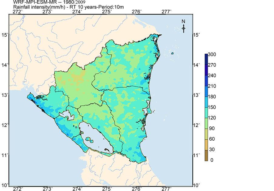
Similar results can be obtained from the comparison of rainfall intensity maps (Figure 16). There is a clear upward trend in the rainfall intensity in the projection period, being more significant in the Departments of Carazo, Chinandega, León and Managua for low durations (10 minutes and 1 hour). Finally, in the case of the duration of 5 days we also observe a significant increase in the rainfall intensity, being more significant in all Departments of the Pacific coast.
5. Conclusions
In this paper climate change projections over Nicaragua have been obtained and analyzed. This work has focused on the achievement of future climate projections of temperature and precipitation over Nicaragua with a thirty years horizon. The aim to do these projections is to prepare and adapt the infrastructures of the country to the effects of climate change, thereby increasing resilience to this phenomenon.
To do this, we have designed a dynamical downscaling methodology based on the coupling of global and regional models. We have followed steps that have enabled us to minimize the uncertainty of the method and to customize the methodology to Nicaraguan features, being the first time that a mesoscale model is used in the country. By comparison with satellite data information we have concluded that MPI-ESM-MR is the global climate model that best reproduces the atmospheric conditions of Nicaragua, obtaining high correlation coefficients for monthly average temperature and monthly precipitation using satellite data. In the same way, the resulting root mean square error is 0.32˚C and 31 mm for monthly average temperature and accumulated precipitation respectively. RCP4.5 has been chosen as the most convenient radiative scenario, being the scenario that agrees with the current world climate agreements. Anyway, the selection of one or another scenario is not relevant
 (a)
(a) (b)
(b) (c)
(c)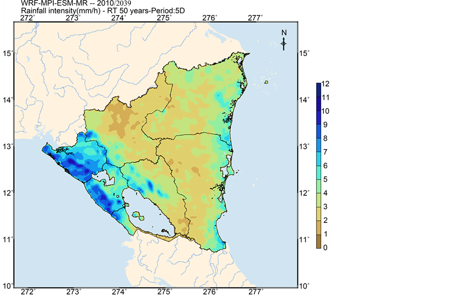 (d)
(d)
Figure 16. Maps of rainfall intensity corresponding to a return period of 10 years and temporal lenght of 10 minutes ( (a) and (b) refers to historical and projected period respectively) and corresponding to a return period of 50 years and temporal length of 5 days ( (c) and (d) refers to historical and projected period respectively).
because their 8-radiative forcing is very similar for the next 30 years.
On the other hand, WRF-ARW mesoscale model has been configured, tested and evaluated over Nicaragua. Using a representative period, we have selected the optimum WRF configuration, and we have been able to reduce monthly average precipitation model uncertainty up to 52%, in comparison with the results obtained using a configuration based on default options. We conclude that cumulus and planetary boundary layer schemes are the most influencing parameterizations in terms of temperature and precipitation accuracy. Tiedtke, as cumulus scheme, and ACM2, as PBL scheme, have been found to be the ones that minimize the model uncertainty of temperature and precipitation in Nicaragua. Working with this optimum configuration and comparing model output and observed values during a 30-year period, 1980-2009, we have obtained correlation coefficients of 0.72 and 0.91, and root mean square errors of 2.0˚C and 113 mm, for monthly average precipitation and monthly average temperature respectively, using information from 148 meteorological stations.
To analyze the climate change signal we have compared mesoscale simulations with a 4 km horizontal resolution covering all Nicaragua for a historical period, 1980-2009, and for a projected period, 2010-2040. Results indicate that an increase in temperature between 0.6˚C and 0.8˚C is expected. This increase will affect all the country, with special relevance in the north. Higher temperatures will affect the number of days with temperatures higher than 35˚C. Results show an increment of this parameter, more important in the north and during the wet period (May to October).
Regarding the precipitation, we observe changes in the monthly precipitation patterns in the regions of the Pacific, increasing the value of the accumulated precipitation at the beginning and at the end of the wet period, and reducing the same value at the inner months. However, the annual precipitation is similar, without significant changes, and within year-to-year variability. Furthermore, an increment of the number of dry days (defined as those without precipitation-0 mm) between 5% and 10% is expected, being more significant during the dry period (November to April). And from the analysis of the IDF curves, we conclude that an increment of the rainfall intensity is expected. We have observed higher 10-minute, 30-minute and hourly rainfall (between 3 and 10%) for the return periods of 10, 25 and 50 years. In the Caribbean regions, the IDF curves for 25 years in the projected period are very similar to the same curve for 50 years in the historical period. This means that the same rainfall intensity will be more frequent in the future.
Acknowledgements
This work has been developed within the framework of the contract ES-007-2015 funded by the Nordic Development Fund and partly funded by the Spanish Government through PTQ-12-05244. Authors are especially grateful to Dr. José Antonio Milán and Eng. Marcio Baca from the Nicaraguan Institute of Territorial Studies for their valuable cooperation and support and for providing meteorological measurements. The authors gratefully acknowledge the technicians at the Ministry of Transport and Infrastructures of the Government of Nicaragua, IDOM consultants, the Nordic Development Fund and Mr. Eduardo Acuña for their collaboration and support.
Cite this paper
Josep Maria Solé,Raúl Arasa,Miquel Picanyol,Mª Ángeles González,Anna Domingo-Dalmau,Marta Masdeu,Ignasi Porras,Bernat Codina, (2016) Assessment of Climate Change in Nicaragua: Analysis of Precipitation and Temperature by Dynamical Downscaling over a 30-Year Horizon. Atmospheric and Climate Sciences,06,445-474. doi: 10.4236/acs.2016.63036
References
- 1. IPCC (2007) Climate Change 2007: The Physical Science Basis. Contribution of Working Group I to the Fourth Assessment Report of the Intergovernmental Panel on Climate Change. Cambridge University Press, Cambridge, United Kingdom and New York, NY, USA.
- 2. Harmeling, S. and Eckstein, D. (2012) Global Climate Risk Index 2013. Who Suffers Most from Extreme Weather Events? Weather-Related Loss Events in 2011 and 1992 to 2011. German Watch, Bonn and Berlin, Germany, 28 p.
- 3. De Loma-Ossorio, E., García, R.A., Córdoba, M. and Ribalayagua, J. (2014) Escenarios del climafuturo para maíz y frijol. Caminos para La adaptación en Nicaragua. Instituto de Estudios del Hambre, Madrid, Spain.
- 4. De Loma-Ossorio, E., García, R.A., Córdoba, M. and Ribalayagua, J. (2014) Estrategias de adaptación al cambio climático em municípios de Nicaragua del Golfo de Fonseca. Instituto de Estudios del Hambre, Madrid, Spain.
- 5. Rapidel, B., Beer, J., Haggar, J., Lader, P., Roupsard, O., Zelaya, C., Gamboa, H., Munguía, R., Ramírez, J. and Vásquez, N. (2013) Respuesras y adaptación del café al cambio climatic en Centroamérica. BID Fontagro. FTG/RF-1027-RG.
http://repository.iadb.org/sites/default/files/stecnico/pp_POA_10_67_2011.pdf - 6. López, C. and Milán, J.A. (2008) Escenarios futures de cambio climatico basados en modelación MARENA. Centro de Investigación y Educación en Cambio Climático.
http://www.cambioclimaticoytecnologia.org/ebook-escenarios-cambio-climatico/Default.html - 7. Wang, Y., et al. (2004) Regional Climate Modeling: Progress, Challenges and Prospects. Journal of the Meteorological Society of Japan, 82, 1599-1628.
http://dx.doi.org/10.2151/jmsj.82.1599 - 8. Pal, J.S., et al. (2007) Regional Climate Modeling for the Developing World: The ICTP RegCM3 and RegCNET. Bulletin of the American Meteorological Society, 88, 1395-1409.
http://dx.doi.org/10.1175/BAMS-88-9-1395 - 9. Hewitson, B.C. and Crane, R.G. (1996) Climate Downscaling: Techniques and Application. Climate Research, 7, 85-95.
http://dx.doi.org/10.3354/cr007085 - 10. Wiley, R.L., et al. (2004) Guidelines for the Use of Climate Scenarios Developed from Statistical Downscaling Methods. IPCC Task Group on Data and Scenario Support for Impact and Climate Analysis (TGICA).
- 11. Giorgi, F. (2006) Regional Climate Modeling: Status and Perspectives. Journal de Physique, 139, 101-118.
http://dx.doi.org/10.1051/jp4:2006139008 - 12. Giorgi, F. and Mearns, L.O. (1999) Introduction to Special Section: Regional Climate Modeling Revisited. Journal of Geophysical Research, 104, 6335-6352.
http://dx.doi.org/10.1029/98JD02072 - 13. Lorenz, P. and Jacob, D. (2005) Influence of Regional Scale Information on the Global Circulation: A Two-Way Nesting Climate Simulation. Geophysical Research Letters, 32, Article ID: L14826.
http://dx.doi.org/10.1029/2005GL023351 - 14. Gao, X., Pal, J.S. and Giorgi, F. (2006) Projected Changes in Mean and Extreme Precipitation over the Mediterranean Region from High Resolutions Double Nested RCM Simulations. Geophysical Research Letters, 33, Article ID: L03706.
http://dx.doi.org/10.1029/2005GL024954 - 15. Hong S.-Y. and Kanamitsu M. (2014) Dynamical Downscaling: Fundamental Issues from an NWP Point of View and Recommendations. Asia-Pacific Journal of Atmospheric Sciences, 50, 83-104.
http://dx.doi.org/10.1007/s13143-014-0029-2 - 16. Hidalgo, H.G. and Alfaro, E.J. (2014) Skill of CMIP5 Climate Models in Reproducing 20th Century Basic Climate Features in Central America. International Journal of Climatology, 35, 3397-3421.
http://dx.doi.org/10.1002/joc.4216 - 17. Van Vuuren, D., Den Elzen, M., Lucas, M., Eickhout, B., Strengers, B., Van Ruijven, B., Wonink, S. and Van Houdt, R. (2007) Stabilizing Greenhouse Gas Concentrations at Low Levels: An Assessment of Reduction Strategies and Costs. Climatic Change, 81, 119-159.
http://dx.doi.org/10.1007/s10584-006-9172-9 - 18. Clarke, L., Edmonds, J., Jacoby, H., Pitcher, H., Reilly, J. and Richels, R. (2007) Scenarios of Greenhouse Gas Emissions and Atmospheric Concentrations. Sub-Report 2.1A of Synthesis and Assessment Product 2.1 by the U.S. Climate Change Science Program and the Subcommittee on Global Change Research. Department of Energy, Office of Biological & Environmental Research, Washington DC, USA, 154 p.
- 19. Fujino, J., Nair, R., Kainuma, M., Masui, T. and Matsuoka, Y. (2006) Multi-Gas Mitigation Analysis on Stabilization Scenarios Using AIM Global Model. Multigas Mitigation and Climate Policy. The Energy Journal.
http://dx.doi.org/10.5547/issn0195-6574-ej-volsi2006-nosi3-17 - 20. Hijioka, Y., Matsuoka, Y., Nishimoto, H., Masui, M. and Kainuma, M. (2008) Global GHG Emissions Scenarios under GHG Concentration Stabilization Targets. Journal of Global Environmental Engineering, 13, 97-108.
- 21. Riahi, K., Gruebler, A. and Nakicenovic, N. (2007) Scenarios of Long-Term Socio-Economic and Environmental Development under Climate Stabilization. Technological Forecasting and Social Change, 7, 887-935.
http://dx.doi.org/10.1016/j.techfore.2006.05.026 - 22. Skamarock, W., Klemp, J., Dudhia, J., Gill, D., Barker, D., Duda, M., Huang, X.-Y., Wang, W. and Powers, J. (2008) A Description of the Advanced Research WRF Version 3. NCAR Tech. Note, NCAR/TN-475+STR.
- 23. Arasa, R., Soler, M.R. and Olid, M. (2012) Numerical Experiments to Determine MM5/WRF-CMAQ Sensitivity to various PBL and Land-Surface Schemes in North-Eastern Spain: Application to a Case Study in Summer 2009. International Journal of Environment and Pollution, 48, 105-116.
http://dx.doi.org/10.1504/IJEP.2012.049657 - 24. Reboredo, B., Arasa, R. and Codina, B. (2015) Evaluating Sensitivity to Different Options and Parameterizations of a Coupled air Quality Modelling System over Bogotá, Colombia. Part I: WRF Model Configuration. Open Journal of Air Pollution, 4, 47-64.
http://dx.doi.org/10.4236/ojap.2015.42006 - 25. Hong, S.-Y. and Lim, Y.-O. (2006) The WRF Single-Moment 6-Class Microphysics Scheme (WMS6). Journal of the Korean Meteorological Society, 42, 129-151.
- 26. Chen, F. and Dudhia, J. (2001) Coupling an Advanced Land-Surface Hydrology Model with the Penn State-NCAR MM5 Modeling Syste. Part I: Model Implementation and Sensitivity. Monthly Weather Review, 129, 569-585.
http://dx.doi.org/10.1175/1520-0493(2001)129<0569:CAALSH>2.0.CO;2 - 27. Collins, W.D., Rasch, P.J., Boville, B.A., Hack, J.J., McCaa, J.R., Williamson, D.L., Kiehl, J.T., Bitz, C., Lin, S.J., Zhang, M. and Dai, Y. (2004) Description of the NCAR Community Atmosphere Model (CAM3.0). NCAR Tech Note, NCAR/TN-464+STR.
- 28. Knievel, J.C., Bryan, G.H. and Hacker, J.F. (2007) Explicit Numerical Diffusion in the WRF Model. Monthly Weather Review, 135, 3808-3824.
http://dx.doi.org/10.1175/2007MWR2100.1 - 29. Saha, S., et al. (2010) The NCEP Climate Forecast System Reanalysis. Bulletin of American Meteorological Society, 91, 1015-1057.
http://dx.doi.org/10.1175/2010BAMS3001.1 - 30. Hong, S.-Y., Noh, Y. and Dudhia, J. (2006) A New Vertical Diffusion Package with an Explicit Treatment of Entrainment Processes. Monthly Weather Review, 134, 2318-2341.
http://dx.doi.org/10.1175/MWR3199.1 - 31. Kain, J.S. (2004) The Kain-Fritsch Convective Parameterization: An Update. Journal of Applied Meteorology, 43, 170-181.
http://dx.doi.org/10.1175/1520-0450(2004)043<0170:TKCPAU>2.0.CO;2 - 32. Zheng, Y., Alpaty, K., Herwehe, J.A., Del Genio, A.D. and Niyogi, D. (2015) Improving High-Resolution Weather Forecasts Using the Weather Research and Forecasting (WRF) Model with an Updated Kain-Fristsch Scheme. Monthly Weather Review, 144, 833-860.
- 33. Grell, G.A. and Devenyi, D. (2002) A Generalized Approach to Parameterizing Convection Combining Ensemble and Data Assimilation Techniques. Geophysical Research Letters, 29, 1693.
http://dx.doi.org/10.1029/2002gl015311 - 34. Han, J. and Pan, H.L. (2011) Revision of Convection and Vertical Diffusion Schemes in the NCEP Global Forecast System. Weather Forecast, 26, 520-533.
http://dx.doi.org/10.1175/WAF-D-10-05038.1 - 35. Zhang, C., Wang, Y. and Hamilton, K. (2011) Improved Representation of Boundary Layer Clouds over the Southeast Pacific in ARW-WRF Using a Modified Tiedtke Cumulus Paramterization Scheme. Monthly Weather Review, 139, 3489-3513.
http://dx.doi.org/10.1175/MWR-D-10-05091.1 - 36. Janjic, Z.I. (1994) The Step-Mountain Eta Coordinate Model: Further Developments of the Convection, Viscous Sublayer and Turbulence Closure Schemes. Monthly Weather Review, 122, 927-945.
http://dx.doi.org/10.1175/1520-0493(1994)122<0927:TSMECM>2.0.CO;2 - 37. Zhang, G.J. and Mu, M. (2005) Effects of Modifications to the Zhang-McFarlane Convection Parameterization on the Simulation of the Tropical Precipitation in the National Center for Atmospheric Research Community Climate Model, Version 3.
- 38. Sukoriansky, S., Galperin, B. and Perov, V. (2005) Application of a New Spectral Theory of Stable Stratified Turbulence to the Atmospheric Boundary Layer over Sea Ice. Boundary-Layer Meteorology, 117, 231-257.
http://dx.doi.org/10.1007/s10546-004-6848-4 - 39. Pleim, J.E. (2007) A Combined Local and Non-Local Closure Model for the Atmospheric Boundary Layer. Part I: Model Description and Testing. Journal of Applied Meteorology and Climatology, 46, 1383-1395.
http://dx.doi.org/10.1175/JAM2539.1 - 40. Nakanishi, M. and Niino, H. (2006) An Improved Mellor-Yamada Level 3 Model: Its Numerical Stability and Application to a Regional Prediction of Advection Fog. Boundary-Layer Meteorology, 119, 397-407.
http://dx.doi.org/10.1007/s10546-005-9030-8 - 41. Bretherton, C.S. and Park, S. (2009) A New Moist Turbulence Parameterization in the Community Atmosphere Model. Journal of Climate, 22, 3422-3448.
http://dx.doi.org/10.1175/2008JCLI2556.1 - 42. Grenier, H. and Bretherton, C.S. (2001) A Moist PBL Parameterization for Large-Scale Models and Its Application to Subtropical Cloud-Topped Marine Boundary Layers. Monthly Weather Review, 129, 357-377.
http://dx.doi.org/10.1175/1520-0493(2001)129<0357:AMPPFL>2.0.CO;2 - 43. Shing, H.H. and Hong, S.-Y. (2015) Representation of the Subgrid-Scale Turbulent Transport in Convective Boundary Layers Resolutions. Monthly Weather Review, 143, 250-271.
http://dx.doi.org/10.1175/MWR-D-14-00116.1 - 44. Leung, L.R., Mearns, L.O., Giorgi, F. and Wilby, R.L. (2003) Regional Climate Research. Bulletin of the American Meteorological Society, 84, 89-95.
http://dx.doi.org/10.1175/BAMS-84-1-89 - 45. Quian, J.-H., Seth, A. and Zebiak, S.E. (2003) Reinitialized versus Continuos Simulations for Regional Climate Downscaling. Monthly Weather Review, 131, 2857-2874.
http://dx.doi.org/10.1175/1520-0493(2003)131<2857:RVCSFR>2.0.CO;2 - 46. Lo, J.C.-F. and Yang, Z.-L. (2007) Comparison of Two Approaches to Dynamical Regional Climate Downscaling Using the WRF Model. Journal of Climate.
- 47. Pan, Z., Takle, E.S., Gutowski, W.J. and Turner, R.W. (1999) Long Simulation of Regional Climate as a Sequence of Short Segments. Monthly Weather Review, 127, 308-321.
http://dx.doi.org/10.1175/1520-0493(1999)127<0308:LSORCA>2.0.CO;2 - 48. Roads, J., Chen, S.-C. and Kanamitsu, M. (2003) U.S. Regional Climate Simulations and Seasonal Forecasts. Journal of Geophysical Research, 108, 8606.
http://dx.doi.org/10.1029/2002JD002232 - 49. Zhang, Z., Qiu, C. and Wang, C. (2008) A Piecewise-Integration Method for Simulating the Influence of External Forcing on Climate. Progress in Natural Science, 18, 1239-1247.
http://dx.doi.org/10.1016/j.pnsc.2008.05.003 - 50. Lucas-Picher, P., Christensen, F. and Berg, P. (2013) Dynamical Downscaling with Reinitializations: A Method to Generate Finescale Climate Datasets Suitable for Impact Studies. Journal of Hydrometeorology, 14, 1159-1174.
http://dx.doi.org/10.1175/JHM-D-12-063.1 - 51. Témez, J. (1978) Cálculo hidrometeorológico de caudales máximos en pequeñas cuencas naturals. Dirección General de Carreteras. Madrid, Spain. 111 p.
- 52. Coles, S. (2001) An Introduction to Statistical Modeling of Extreme Values. Springer-Verlag, London.
http://dx.doi.org/10.1007/978-1-4471-3675-0 - 53. Guvareva, T.S. and Garstman, B.I. (2010) Estimating Distribution Parameters of Extreme Hydrometeorological Characteristics by L-Moment Method. Water Resources, 37, 437-445.
http://dx.doi.org/10.1134/S0097807810040020