Agricultural Sciences
Vol.08 No.09(2017), Article ID:78999,12 pages
10.4236/as.2017.89070
Positioning Temperature Sensors for Frost Protection in Northern Cranberry Production
Vincent Pelletier, Silvio Jose Gumiere*, Steeve Pepin, Jacques Gallichand, Jean Caron
Département des Sols et de Génie Agroalimentaire, Université Laval, Québec, Canada

Copyright © 2017 by authors and ScientificResearch Publishing Inc.
This work is licensed under the CreativeCommons Attribution International License (CC BY 4.0).
http://creativecommons.org/licenses/by/4.0/


Received: July 7, 2017; Accepted: September 8, 2017; Published: September 12, 2017
ABSTRACT
Frost can cause serious economic losses in cranberry fields, particularly in northern regions. When the air temperature reaches a low critical threshold, sprinklers are operated to protect vines, to insure crop production and profitability. To avoid frost injury, proper positioning of temperature sensors is critical. A field experiment was designed and conducted to determine the optimal installation height of sensors above soil surface. Temperature data was used to investigate the spatial temperature gradient in the section of a cranberry field. A computer simulation of the temperature profile was performed to simulate the effect of wind velocity on the prediction of air temperature. For optimal use, sensors should be installed at the height of the canopy and several meters away from a dike. On nights with low wind velocities, the canopy air temperature was 2.7˚C below that of 500 cm above the ground. The sensors should be put at least five m away from a dike to avoid the transfer of heat from the dike to the sensor. Also, multiple sensors should be installed because of the large variations in air temperature that were measured across the experiment. The simulated temperature indicated that wind velocity strongly influenced the temperature estimation; the effect of the wind on temperatures gradients was greater when the wind velocity was low (<2.3 m/s).
Keywords:
Frost Protection, Cranberry Production, Numerical Simulation of Heat Transfer

1. Introduction
The USA and Canada are the leaders in the production of cranberries, producing 98% of the world’s crop [1] . In the northern regions of North America, cranberries grow naturally in peat bogs, in which the thermal flow from the subsoil typically keeps the temperature of the plants above 0˚C even when the air temperature drops down to −10˚C [2] . Cranberries are intensively cultivated in sandy soils, and on cold spring nights, low temperatures may kill buds, flowers and plant tissue depending upon temperature and duration.
In many crops, buds and flowers are most vulnerable to freeze damage. Cold is the primary factor that limits agricultural production in temperate areas [3] . Frost protection is one of the most important cultural practices in the production of cranberries [4] . Although flooding is used for protection from winter frost, sprinklers are typically used in the spring, summer and fall to protect the plants. Field temperatures are stabilized from the heat released by the freezing water. Following 17 cold nights, [5] found yield losses of 90% and a 15% reduction in the size of the berries in unprotected beds compared to berries in sprinkled beds. For unprotected vines, major losses occur when the frost persists for only one hour [4] . The critical air temperature threshold to begin irrigation is dependent on the cultivar and on the stage of growth. For example, with the ‘Stevens’ cultivar, the tolerance threshold is −5˚C at the cabbage head stage, −3˚C at the bud elongation stage, and −1˚C during the hook and bloom stage [6] . At a temperature of −2˚C, [7] found that 9% of the flowers died, whereas at −4˚C and −6˚C, the mortality of the flowers reached 45% and 76%, respectively. Similar results were found in cherries for which a difference of 1˚C (i.e. exposure for several hours to −6˚C vs −7˚C) resulted in the mortality of twice as many blooms [8] . In peaches, protection from frost with sprinklers resulted in a 12% blossom kill compared with 42% in a nonsprinkled area [9] . With grape wines, frost protection is essential to avoid the damaging effect of cold events [10] .
[10] and [11] recognized three types of cold spring nights. Radiation frost occurs on nights with clear skies and calm winds of less than 2.2 m/s, and this type of cold event is caused by radiational heat losses from the ground and solid objects (e.g. cranberry shoots), which results in an increase in air temperature with elevation above the crop. On advective freezing nights, when the winds exceed 4.5 m/s, a dangerous weather event can be anticipated with subfreezing temperatures that are associated with a large frontal system of cold air over an entire region. The third type of cold spring night is a combination of frost and freezing temperatures when the wind is between 2.2 and 4.5 m/s. Cranberry growers noticed that for most of the nights requiring frost protection wind velocity was low. Freezing nights can be catastrophic because sprinklers are not effective when the air temperature is below −8˚C.
Traditional frost protection management systems use wired sensors installed a few meters from the dikes; when a critically low temperature is reached those sensors send an alarm via a phone line. The newer generation of frost protection systems includes real-time temperature monitoring and automated pumps that start when air temperature reaches the critical threshold. Monitoring of temperatures must be accurate and representative of the cranberry field to avoid frost injuries; overestimation of temperatures could result in irreversible tissue injuries, whereas underestimation could result in large amounts of water losses, pumping energy, and unnecessary operational costs. For frost protection, sprinklers apply approximately 300 - 400 m3∙ha−1 of water on a typical night.
The cranberry guide [4] recommends that temperature sensors be installed at the top of the vines; however, there is no documentation from the literature to support this recommendation. Additionally, despite that recommendation, our own survey showed that some growers install their temperature probes at different heights, which varied from into the vines to one meter above the canopy. Although these growers are convinced that their sensors are correctly located, an incorrect positioning of the temperature probes within the vertical profile above the cranberry field would bias the temperature measurements and could lead to significant damages to the crop.
This study was performed in two phases: a field experiment and a computer simulation. The field experiment was to determine the best vertical position of temperature probes in the field for frost control decisions. The second part was designed to investigate the effects of the dikes and wind velocities on the temperature distribution profile across a cranberry field.
2. Materials and Methods
2.1. Field Experiment
2.1.1. Experimental Site
The field experiment was conducted in four adjacent cranberry beds (46˚17'N; 71˚59'W) located in the Canadian province of Québec (Figure 1(a)). A sodded dike, 1 m high and 7 m wide with a 1:1 slope, separated each bed (52 m × 480 m) and was used for machinery circulation. Three irrigation lines were buried in each bed with a sprinkler spacing of 15 m. The first and last irrigation lines were located 8 m from a dike, and the middle line was in the center of the bed. With a pressure of 350 kPa at the sprinkler heads, water application was uniform with an application rate of 4.5 mm/h. According to the 1971-2000 climatic (Environ-

Figure 1. (a) Location of the field experiment in Canada; (b) positions of the temperature towers; (c) temperature probes installed across the width of a bed.
nement Canada), the normal maximum, average and minimum temperatures for the spring months in this area are 1.2, −4.0 and −9.2˚C in March; 9.7, 4.3 and −1.0˚C in April; 17.6, 11.4 and 5.3°C in May; and 22.6, 16.7 and 10.8˚C in June, respectively.
2.1.2. Measurements
For the field experiment, eight measurement towers were installed in the beds (Figure 1(b)) with each one recording air temperature at four heights: the midpoint of the vines (6 cm above ground), in the vicinity of the buds (12 cm above ground) and two positions above the canopy (25 and 50 cm above ground). Three of the towers were equipped with copper-constantan thermocouples, and five of the towers were equipped with TAM model thermistors (Hortau, Lévis, Canada). There were no significant differences in temperature readings between the thermocouples and thermistors (unpublished data). The readings from the thermocouples were recorded with data loggers (CR10X; Campbell Scientific, Edmonton, Canada), and the readings from the thermistors were processed via a wireless communication system to the Irrolis Website (http://www.hortau.com/, Lévis, Canada). The climatic data were collected at 15-min intervals with an Irrolis automated weather station (Hortau, Lévis, Canada) installed 2 m above the ground and 500 m from the experimental beds. From 20 April 2012 to 16 May 2012, contrast analyses were conducted separately for six calm nights (wind < 2.2 m/s) and for five turbulent nights (wind > 2.2 m/s). Twenty TAM temperature probes (Hortau, Lévis, Canada) were installed 12.5 cm above ground in a bed at a 2.75 m spacing to monitor the effect of the dikes on heat transfer (Figure 1(c)). There was no frost irrigation on the nights that were monitored with the 20 sensors.
2.2. Computer Simulation
2.2.1. Airflow
To calculate the airflow over the field, we used the compressible flow approximation, in which variations in air density are calculated as a function of flow velocity. For the inflow profile of the wind velocity, we considered time-dependent solutions for constant boundary conditions. When body forces, such as buoyancy, were ignored, the airflow over the field was described with the Navier-Stokes (NS) and continuity equations with laminar flow [12] . Nevertheless, surface turbulence can influence the transport and exchange of heat between the surface and atmosphere [13] but was not considered in this study. Assuming laminar flow conditions, the Newtonian fluid NS-equation and the continuity equation are written as:
(1)
(2)
where ρ [kg∙m−3] is the air density; u [m∙s−1] is the velocity vector in both (x, y) directions; p [Pa] is the air pressure; T [˚C] is the temperature; and µ [Pa s] is the fluid viscosity.
2.2.2. Heat Transfer in Fluids
The transfer of energy in the air domain over the field surface is described by Equation (3) [14] as follows:
(3)
where ρ [kg∙m−3] is the air density; u [m∙s−1] is the velocity vector in both (x, y) directions; Cp [J∙kg−1∙K−1] is the specific heat capacity at constant temperature; T [˚C] is the temperature and k [W∙m−1∙K−1] is the thermal conductivity, which is considered isotropic for the domain.
2.2.3. Boundary Conditions
Airflow: To solve this aerodynamic problem, we specified the appropriate boundary conditions (Figure 2); there are four types of boundaries in this problem. The inflow boundary is on the left side from which airflow enters the domain with a constant parabolic velocity profile. The vertical velocity flow component is zero because the wind blows across a wide, flat region (5 m) before the embankment, at which point the even flow was disturbed. On the right side, an outflow boundary condition is set from which air flows out of the domain. Assumed to be free, the outflow is controlled only by the pressure gradient that is generated inside the domain. At the internal bottom of the domain, a wall with a no-slip (u = 0) condition was used and, at the top, we consider the boundary condition to be open. The initial condition is to u = 0 for the entire domain at t = 0.
Heat transfer: We use only two types of boundary conditions for the heat transfer differential equation. For the left, bottom and right boundaries, the thermal insulation boundary conditions is set to zero inward heat flux normal to the boundary. For the upper boundary, a constant temperature boundary condition is chosen to account for the effects of atmospheric temperatures. For the

Figure 2. Boundary and initial conditions for the temperature profile simulations.
initial condition, we set a constant temperature of 2˚C for the entire domain at t = 0.
3. Results and Discussion
3.1. Field Experiment
3.1.1. Optimal Installation Height for Temperature Sensors
The climatic data for the eleven nights are shown in Table 1. On both types of night (calm and turbulent), the coldest position was 12 cm above the ground, near the buds (Table 2). On calm nights, the temperature was significantly higher at 6, 25, and 50 cm above the ground than at canopy height (12 cm above ground). The average temperature at 12 cm was 1.43˚C colder than at 50 cm

Table 1. Weather conditions for 11 nights (from 20 April 2012 to 16 May 2012) in a cranberry field (C: Calm; T: Turbulent; RH: relative humidity; Patm: atmospheric pressure) (m∙s−1)
Table 2. Statistical comparison of air temperature at 6, 25, and 50 cm height above ground vs temperature at canopy height (12 cm above the ground). Mean air temperature at each height is the average of n nights and was computed from measurements carried out between midnight and 5:45.
zNS = Not significantly different from temperature at 12 cm.
above the ground (Table 2). The greatest difference in temperature recorded between two heights simultaneously was 4.4˚C, when the temperature was −0.3˚C at 12 cm and 4.1˚C at 50 cm above ground. The differences in air temperature with height were not significant on turbulent nights. The temperature distributions on one typical calm laminar night and one typical turbulent night are shown in Figure 3. The temperature dropped rapidly from 6.1˚C at 00:00 to −0.1˚C three hours later at 12 cm above the ground on a calm night. When the minimum temperature was reached at 12 cm, the temperatures at 6, 25, and 50 cm above the ground were on average 0.7˚C, 0.9˚C and 1.6˚C higher than at 12 cm, respectively. This has an important impact. If the temperature threshold to start irrigation had been set at 1.0˚C on that night, the irrigation would have started at 02:15 based on measurements from the sensors installed at bud height.
 (a)
(a) (b)
(b)
Figure 3. Temperature profile above the ground (4 heights: 6 cm (grey); 12 cm (black); 25 cm (dashed); and 50 cm (pointed)) at 7 towers and the weather conditions at the weather station for one calm (a) and one turbulent night (b). (a) Typical calm night (Night 1 in Table 2); (b) typical turbulent night (Night 2 in Table 2).
If the sensors were installed at 25 cm above the ground, the irrigation would have been delayed by 195 min, whereas no frost protection would have been required based on temperature readings at 6 and 50 cm above the ground. On a typical turbulent night, when the minimum temperature was reached at 12 cm above ground, the average temperatures at 6, 25, and 50 cm were 0.1˚C, 0.1˚C, and 0.2˚C higher than that at 12 cm, respectively, and the temperatures remained largely stable between 00:00 and 06:00. The rapid decline in temperature on calm nights reflects the importance for growers to rely on a system for which data are rapidly transmitted instead of relying on manual readings. With automation, a difference as small as 0.1˚C would determine whether or not start the irrigation for frost protection. Sensors that are misplaced could lead to unprotected vines when protection is required.
3.1.2. Spatial Variation in Air Temperature across the Field
Although the towers were installed in the same block of beds, large spatial differences were measured. Considering only the height of 12 cm above the ground for a laminar night (Figure 3(a)) with a critical threshold at 2˚C, a 30 min delay at the start of irrigation would have occurred between the lowest (Tower #1) and highest temperatures (Tower #7); the temperature at Tower #1 had decreased to 0.1˚C by the time the temperature at Tower #7 reached the critical threshold of 2˚C. At the same moment, the temperature at the weather station (2 m above ground) was 6.4˚C and never dropped below 2˚C. If the grower used only one probe, or worse, if the grower used only a local weather station, the situation would have resulted in frost damage in the colder areas of the bed. This situation demonstrates the importance of having multiple temperature sensors in cranberry fields. Because a small duration of frost can cause important physiological damages, multiple sensors coupled to a spatially distributed automated irrigation system could avoid frost injuries and reduce the amount of water required for frost protection resulting in economical and environmental benefits. Further research is required to determine the optimum number of probes to be installed in each area.
3.1.3. Air Temperature Variations across a Bed
The relationship between the temperature and the distance from the ditch was investigated on 13 spring nights with probes placed 12.5 cm above the ground. For 8 of these nights, the relationship corresponded to a significant (p < 0.05) quadratic function of the form , where T is the temperature and x the distance from the dike. Figure 4 shows the relationship between the parameter “a” and wind velocity. Decreasing values of “a” with wind speed indicates that the dikes play an important role in the temperature pattern. The effect of dikes on temperature was wind velocity dependent; being greater on calm nights. The difference in temperature between probes located near the dike and those in the center of the bed was also greater on calm nights. On a turbulent night with a high wind velocity (3.5 m∙s−1; Figure 5(a)), the value of “a” was
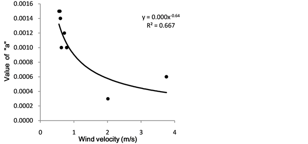
Figure 4. Relationship between the value of “a” (quadratic function of the pattern of temperature with the distance from the dike) and wind velocity.

Figure 5. Temperature distribution pattern with distance from the dike during two typical nights with (a) high and (b) low velocity winds. TWS is the air temperature observed at the weather station. (a) Wind velocity = 3.5 m/s, TWS = 11.1˚C; (b) wind velocity = 0.7 m/s, TWS = 8.3˚C.
small (0.0002) and the difference between the highest and lowest temperatures of the bed was also small (0.6˚C). During a calm night, with low wind velocity (0.7 m∙s−1; Figure 5(b)), the value of “a” (0.0012) was six times higher than that for turbulent night A, and the difference between the highest and lowest temperatures of the bed was high (2.3˚C). For all measured nights, the average difference between the highest and lowest temperatures across the bed (DT) was 1.4˚C ± 0.6˚C, and the correlation with wind velocity (u) was significant and linear (DT = −0.11u + 2.00; p = 0.002). The average difference between temperatures at the on-site weather station and the temperature in the coldest part of the bed was 4.8˚C ± 2.9˚C, and the correlation with the wind was also significant and linear (DT = −0.43u + 7.15; p = 0.03). The relationships between air temperature and both relative humidity and atmospheric pressure were examined, but were not significant.
A small deviation from the actual air temperature, depending on plant growth stage, could damage plants and place buds, flowers, and berries at frost risk. The use of a single temperature sensor located near a dike to initiate frost protection would result in a greater bias on calm nights than on a turbulent night. Because the dikes are higher than the ground of the bed, heat is transferred from the soil of the dike to the plants growing near the dike. Such temperature gradient decreased with increasing distance from the dike and, at the center of the bed, the effect of the dike is negligible. On nights with high winds, heat released from the dike is rapidly dissipated over the bed and the effect across the bed is negligible.
3.2. Temperature Profile Simulations
The temperature profiles for the transverse section of the field are presented in Figure 6 for wind velocities from 1.0 to 3.0 m∙s−1. When the wind velocity is
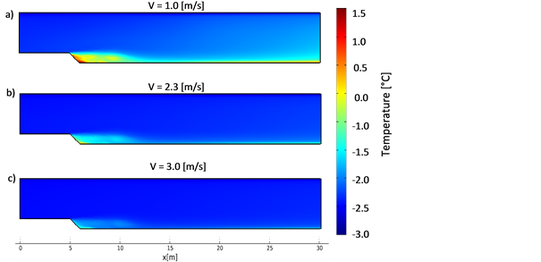
Figure 6. 2D simulated temperature profile across the field with wind velocity equal to: (a) 1.0 m/s; (b) 2.3 m/s; and (c) 3.0 m/s.
1.0 m∙s−1, a strong influence of the dike on the distribution of temperatures is ob- served, likely because the effects of low wind velocity on the mixing and because the wall limit layer effect is small. This relationship would have a strong effect on temperature prediction and frost management if the grower were to place the temperature probe near the edge of the field when the wind velocity is low (u < 2.3 m∙s−1); the grower might have a 1˚C to 2˚C difference compared to the middle of the field. Thus, the grower might overestimate the temperature and choose not to operate sprinklers, causing frost damage to the crop and losses in productivity. When the wind velocity increases (Figure 6(b) and Figure 6(c)), the mixing effect also increases, and the temperature profile is more uniform. Additionally, the wall limit layer effect was not evident, and the difference between the near-dike and mid-field temperatures decreased. The risk of temperature overestimation is lower for high wind velocities (u > 2.3 m∙s−1) than for low wind velocities.
4. Conclusions
The field experiments showed that temperature sensors should be installed at canopy height where the buds are located (~12 cm above ground). The temperature sensors that were installed 50 cm above ground recorded temperatures that were significantly higher than temperatures at 12 cm on low wind nights, with a maximum difference of 4.4˚C. When the sensors were installed close to a dike, the heat from the dike led to higher temperature readings, which could leave unprotected vines further from the dike despite they required frost protection. The variability of temperatures in one block of beds highlighted the importance to have multiple temperature sensors on a farm. Therefore, an automated frost protection system that use multiple sensors installed at the canopy height, could more accurately predict frost risk and conserve water and energy.
The temperature simulations indicated that the wind velocity associated with the wall limit layer might cause an error in the estimation of field temperatures, an error potentially harmful for crop productivity. The errors in the estimation of temperature were more likely when the wind velocity was less than 2.3 m∙s−1. At higher wind velocities, the air is mixed, which effectively homogenizes the temperature profile across the field and reduces the dike protection effect.
Acknowledgements
The authors recognize the financial participation of the Natural Sciences and Engineering Research Council of Canada, Nature Canneberge, Canneberges Bieler, Transport Gaston Nadeau, Hortau, and the Scientific Research and Experimental Development Tax Incentive Program of the Canada Revenue Agency and Revenu Québec.
Cite this paper
Pelletier, V., Gumiere, S.J., Pepin, S., Gallichand, J. and Caron, J. (2017) Positioning Temperature Sensors for Frost Protection in Northern Cranberry Production. Agricultural Sciences, 8, 960-971. https://doi.org/10.4236/as.2017.89070
References
- 1. Bird, R., Stewart, W. and Lightfoot, E. (2002) Transport Phenomena. 2nd Edition, John Wiley, New York.
- 2. Carrer, G. (2014) Dynamique des écoulements et du stockage d’eau d’un petit bassin versant boréal influencé par une tourbière minérotrophe aqualysée des Hautes-terres de la baie de James, Québec, Canada. Thèse. Québec, Université du Québec, Institut national de la recherche scientifique, 320 p.
- 3. Eaton, G.W. (1966) The Effect of Frost upon Seed Number and Berry SIZE in the cranberry. Canadian Journal of Plant Science, 46, 87-88. https://doi.org/10.4141/cjps66-011
- 4. FAOSTAT (2015) Cranberries - Production of Top 5 Producers in 2013. Food and Agriculture Organization of the United Nations - Statistics Division.
- 5. Ghaemi, A.A., Rafie, M.R. and Sepaskhah, A.R. (2009) Tree-Temperature Monitoring for frost Protection of Orchards in Semi-Arid Regions Using Sprinkler Irrigation. Agricultural Sciences in China, 8, 98-107. https://doi.org/10.1016/S1671-2927(09)60014-6
- 6. Holman, J.P. (2010) Heat Transfer. Mcgraw-Hill, New York.
- 7. Ishihara, Y., Shimojima, E. and Harada, H. (1992) Water Vapor Transfer Beneath Bare Soil Where Evaporation Is Influenced by a Turbulent Surface Wind. Journal of Hydrology, 131, 63-104. https://doi.org/10.1016/0022-1694(92)90213-F
- 8. Perry, K.B. (1998) Basics of Frost and Freeze Protection for Horticultural Crops. HortTechnology, 8, 10-15.
- 9. Poling, E.B. (2008) Spring Cold Injury to Winegrapes and Protection Strategies and Methods. HortScience, 43, 1652-1662.
- 10. Rodrigo, J. (2000) Spring Frosts in Deciduous Fruit Trees—Morphological Damage and Flower Hardiness. Scientia Horticulturae, 85, 155-173. https://doi.org/10.1016/S0304-4238(99)00150-8
- 11. Reader, R.J. (1979) Flower cold Hardiness: A Potential Determinant of the Flowering Sequence Exhibited by Bog Ericads. Canadian Journal of Botany, 57, 997-999. https://doi.org/10.1139/b79-123
- 12. Salazar-Gutiérrez, M.R., Chaves, B., Anothai, J., Whiting, M. and Hoogenboom, G., (2014) Variation in Cold Hardiness of Sweet Cherry Flower Buds through Different Phenological Stages. Scientia Horticulturae, 172, 161-167. https://doi.org/10.1016/j.scienta.2014.04.002
- 13. Sandler, H.A. and DeMoranville, C.J. (2008) Cranberry Production: A Guide for Massachusetts, Summary Edition. Cranberry Station - University of Massachusetts Amherst, Amherst.
- 14. Workmaster, B.A. and Palta, J.P. (2009) Frost Hardiness of Cranberry Plants: A Guide to Manage the Crop during Critical Periods in Spring and Fall. Department of Horticulture, University of Wisconsin, 20 p.