Agricultural Sciences
Vol.4 No.8(2013), Article ID:35705,34 pages DOI:10.4236/as.2013.48057
Desirability of a standard notation for fisheries assessment
![]()
Institute for Coastal Marine Environment—IAMC, Italian National Research Council—CNR, Mazara del Vallo, Italy; *Corresponding Author: sergio.vitale@cnr.it
Copyright © 2013 Sergio Ragonese, Sergio Vitale. This is an open access article distributed under the Creative Commons Attribution License, which permits unrestricted use, distribution, and reproduction in any medium, provided the original work is properly cited.
Received 26 April 2013; revised 27 May 2013; accepted 15 June 2013
Keywords: Fisheries; Assessment; Symbols; Standard
ABSTRACT
The worldwide increase of the publications concerning the assessment of marine renewable living resources is highlighting long-standing problems with symbols and annotations. Starting from the symbols presented within the classic fisheries masterpieces produced, mainly in the fifty of the last century, a first “Milestone” list was organised. Thereafter, the pertinent literature was (not exhaustively) browsed in order to integrate this Milestone list on the base of a set of decisional criteria. The present contribution consists in using the Latin letters as well established symbols for the corresponding parameters, leaving free to specific use (with few historical exceptions) the Greek letters in view to open a discussion among all the fisheries scientists and bodies in order to move towards a common language and better communication standards.
1. INTRODUCTION
The intuition to separate out the effects of births, deaths and growth on fish populations in order to estimate the surplus production of an exploitable stock has been developed since the first decades of the twentieth century [1-4]. The origin of fisheries science, as an integrated and structured discipline, however, might be generally placed at the second half of fifties and first half of sixty, when the milestones of Beverton and Holt [5-7], Gulland [8-11], and Ricker [12,13] were published. At that time, the main goals of such discipline were assessing and managing the living renewable aquatic resources under a theoretical based exploitation pattern. Just little after the Beverton and Holt and Ricker works, it was evident the opportunity to be clear about the definition of physical quantities and naming conventions came [14- 16]. Almost half a century later, notwithstanding the growing importance of assessments to promote credible and effective rebuilding or managing plans for the highly depleted fishable resources in the world, on our knowledge no general agreement exists about a proper and unambiguous annotations and symbols. That notwithstanding a big effort has been realised regarding the definitions [17-23]. In the present contribution, which recalls the Holt’s heading of a section in one of his reports presented at the Biarritz symposium in 1956, the most common pitfall, ambiguities and lack of consistency arising from the literature in the field were analysed and a scheme of symbols usage was proposed in order to encourage fisheries scientists and bodies to move towards the establishment of a common language and better communication standards in assessments terminology.
2. MATERIAL AND METHODS
2.1. Organising the Symbols Lists
The pertinent fisheries literature was browsed to highlight the different symbols uses and attributions within a “classic” definition of assessment. In fact, it is worth noting that different assessment interpretations can be found in both grey [24] and “official” publications [25,26] according to a more or less broad application of the word. In particular, within the “broader” interpretations can be quoted 1) the part of fisheries science that studies the status of a fish stock as well as the possible outcomes of different management alternatives; it tells us if the abundance of a stock is below or above a given target point and by doing so lets us know whether the stock is overexploited or not; it also tells us if a catch level will maintain or change the abundance of the stock [27]; and 2) the application of statistical and mathematical tools to relevant data in order to obtain a quantitative understanding of the status of the stock as needed to make quantitative predictions of the stocks reactions to alternative future regimes [22].
On the contrary, the goals of the classic and narrower assessment definitions can be identified in a) for any given fish populations 1) what are the present quantities that will be available for capture in one or more years and what factors are determining the quantity of the fish and how are they changing [28]; 2) providing a means of expressing population properties by a relatively few parameters [26] and of codifying the effects of fishing on stocks [29]; 3) using stock demographic parameters to determine the total catch and how the catch and the catch per unit of effort varies with changes in the pattern of fishing [30]; and 4) the study of population structure, dynamics, and past exploitation of a single population [31] and its reaction to the dominant influence of fishing pressure [32].
Considering the classic definitions, the first step consisted in establishing a “Milestone” list with the historical symbols on the base of the fisheries science masterpieces produced in the fifties and sixties, and integrated with the successive contributes of the same Authors. In particular, the following contributes were consulted: Beverton [33], Beverton and Holt [5-7], Beverton and Parrish [34], Holt [15,35-37], Holt et al. [16], Gulland [8-11,14,24,30,38-45], Gulland and Holt [46], ICNAF [29,47-50], Kesteven and Holt [51], Ricker [12,13,52-58], and Ricker and Foerster [59]. For convenience, these Authors were abbreviated within the Milestone list as BH (Beverton, Holt and Beverton and Holt); I (ICNAF reports), G (Gulland) and R (Ricker).
Hence, the literature (both official and grey), books, manuals and programmes dealing with fisheries assessments were (not exhaustively) consulted in order to compare and integrate the basic scheme previously established. The final step was proposing a standard set of symbols, preferably (or whenever possible) according to the following Decalogue of criteria and conventions [14-16]. In particular, the symbols:
1) should be referred to the most relevant and studies items in “classic” fishery assessment;
2) should have a unique correspondence for each quantity, at least in base of their position (prefix, suffix, subscripts, superscript);
3) should be found within a standard commonly and easily available (in the specific case, the symbols lists in word Microsoft) avoiding other difficult, already existing, to find symbols [60];
4) should avoid special characters, such as the circumflex accent or the “ ” symbol, which was employed for example by Gulland [11,30] with the meaning of “therefore” or “consequently” [60; page 415];
5) should be different from those symbols traditionally well established in other related discipline (such as statistics);
6) in the masterpieces proposals or traditionally established should be maintained;
7) should consist of one to three “components” (never more than four letters), considering that in many instances many subscripts could be necessary [61];
8) should represent the initial words of the considered variable;
9) should help in expressing the relevant formula in a simple and compact form, which is easy to write, type and print;
10) similar should indicate similar measures.
In both Milestone and proposed list, the symbol § and §§ denote some remarks relative to the proposed symbol definition and alternative meanings of the same symbols, respectively. At the beginning of the proposed list, the X symbol was employed to represent some generalisations. Finally, the following abbreviations were adopted: coef. for coefficient, cons. for constant, n˚ for number, par. for parameter, prop. for proportion, and VBGF for von Bertalanffy Growth Function.
2.2. The “Milestone” List
a—BH_ Coef. of linear equations relating growth to density; unit haul swept area; intersect in regression line; const.; time interval (for example, in length increment— average length regression); average (strictly speaking) median length in Tauti’s expression. G_ Probability (in age estimation); slope in the linear density dependence regression between asymptotic length and abundance; coef.; hook catch probability; area or volume under the influence of a gear; prop. of full fishing mortality rate; age at recruitment; proportionality coef. (usually 0.5) among yield, natural mortality and stock biomass (Y = aMB) in potential yield computation. I_ Mesh size. R_ Annual (or seasonal) total mortality rate; annual expectation; actual mortality; the first (multiplier) coef. in the (individual) length-weight functional relationship; coef. in Ricker’s recruitment curve (when stock size and recruitment are in the same units); competition coef.; intercept in regression; sex ratio as males over females; Brody’s coef.; intercept in yield per effort against effort; initial size; cons.
α (alfa)—BH_ Derived coef. of pre recruited mortality in the eggs-recruitment relationship; angle definition; cons. G_ Vulnerability; proportionality coef. R_ Par. in the Ricker (dimensionless) and Beverton and Holt R/S curves.
A—BH_ The area occupied by the fish population; Russell’s recruitment. G_ Sum of squares; coef. in ageing error; area of fished region; Russell’s recruitment; (Heincke’s) annual death rate; cons. in stock recruitment curves. I_ Fish breadth/fish depth ratio. R_ Average population in successive years; annual (also Heincke) or seasonal mortality rate; A' annual or seasonal rate of disappearance of fish; maturity categories n˚ in Murphy’s method; par. in other growth model than VBGF; par. in the Beverton and Holt R/S curve when S and R are in the same units; A0.95 upper age limit according to Taylor’s approximation [62].
b—BH_ Selection factor; ratio of length at 50% point of selection ogive (or mean selection length) to mesh size; coef. of linear equations relating growth to density; Huxley’s coef. in fish length-weight relationship (w = blk); coef. (scale factor) in the Richards curve; coef. in length increment—average length regression; oldest age in Tauti’s expression. G_ Probability (in age estimation); generic coef.; selection factor; density dependence in recruitment; generic slope in linear regression; bn expanding term in the analytical computation. R_ The exponent in the allometric (b ≠ 3) and isometric (b = 3) length-weight (individual) relationship; the slope of any line; proportionality coef. in recruits parental relationships; Brody’s coef.; annual catch in Baranov’s food biomass relationship; intercept in yield-effort (Y/f) against f; cons.
β (beta)—BH_ Derived coef. of pre recruited mortality in the eggs-recruitment relationship; cons. R_ N˚ of marked fish; incomplete beta function; par. in the Ricker and Beverton and Holt R/S curves.
B—G_ Stock biomass (size in weight); sum of squares; coef. in ageing error; biomass, B' in exploited phase; B∞ at maximum population (carrying capacity); BP predators; cons. in stock recruitment curves. I_ Mesh length/mesh width ratio. R_ N˚ of natural death; biomass of a group of fish or an entire stock; maturity categories n˚ in Murphy’s method; par. in other growth model than VBGF; prop. of new recruits in the catch (Allen’s method); B∞ and BS maximum stock size (the environment will support) and “optimum” stock size corresponding to maximum Y at equilibrium in Graham surplus production curve.
c—BH_ Cons. given by the ratio of fishing mortality and “effective overall fishing intensity” (effort); catch per net. G_ Cons.; c' proportionality coef. relating catch per unit of effort to density of fish (provided that the availability is cons.); reciprocal of vulnerability—aggregation product; coef.; ratio of length at capture and maximum length (in potential yield computations); mean selection or entry to the catch or first capture; Y/Ymax ratio in marginal yield analysis; raising factor (from haul catch to stock size). I_ Capture related general par.; Xc at first capture; first liable to capture by the fishing gear in use; tc age at entry to the exploited phase or first liability to capture; selection factor. R_ The catch up to any time; Widrig’s catchability; the fraction of the whole stock captured in a single unit of effort; Brody’s coef.; Xc compensatory component in natural mortality; par. in growth models different from (or previous than) VBGF.
C—BH_ Catch in n˚; local density (concentration) of fish; C’ catch per effort. G_ Catch in n˚; sum of squares; total catch. C1…c species competing with target species; cons. in stock recruitment curves. I_ N˚ of fish in the catch (catch in n˚); head girth/head breadth ratio. R_ Cons. of integration; catch in n˚ (usually in 1 year); n˚ of fish examined for tags or marks; maturity categories n˚ in Murphy’s method; average minimum age limit of usable stock.
χ (chi)—BH_ Fecundity (/g) coef. G_ χ2 chi square statistic.
d—BH_ Average distance of fish in random movement. G_ Catch per unit of effort; sample catch; density of fish as derived in a given haul catch; mean depth. R_ Annual increase in length in Baranov’s Yield method; absolute increase in length.
D—BH_ Dispersion coef.; unconditional natural mortality rate; expectation of death by natural causes; average density of fish. G_ Density of fish on fishing grounds; n˚ dying of disease; cons. in stock recruitment curves. I_ Expectation of death by capture (unconditional natural mortality rate); expectation of death by natural causes. R_ Total deaths; maturity categories n˚ in Murphy’s method.
Δ (delta)—BH_ R_ Interval; variation; change. G_ One or unit operation.
e—G_ Sample effort. R_ Base of the natural (or Napierian) logarithms.
ε (epsilon)—BH_ Coef. of food utilisation for growth and maintenance; efficiency of utilization of food for growth. G_ Coef. in mortality estimation; random variable in fishing effort analysis.
η (eta)—BH_ Suffix denoting reference to spawning or (first) maturity; marked change in growth; cons. in the differential Richards.
E—BH_ G_ I_ R_ Exploitation rate [F/Z(1 − exp−Z)]. BH_ Egg production; XE equilibrium; coef. of anabolism; unconditional fishing mortality rate; expectation of death by capture; par. in the differential length based VBGF; Taylor’s KL∞ product. G_ XE expected value; probability of ultimate capture (often exploitation ratio in steady state condition). I_ Unconditional fishing mortality rate; expectation of death by capture. R_ Escapement; (absolute) n˚ of eggs; XE equilibrium (steady state); cumulative fishing effort.
E.F.—I_ Escape factor as length/mesh size.
f—BH_ Fishing activity; effort; intensity; power; overall; weighed mean fishing effort per unit area. G_ Fishing intensity; fishing effort (in some suitable units); f' adjusted; f(X) function. I_ “Japanese” mortality rate; effective overall fishing intensity. R_ Fishing effort (n˚ of units of gear in use); Widrig’s effective fishing effort adjusted, when necessary; fS corresponding to MSY (optimum f).
♀—R_ Females (reproducing the Petersen 1892 table). I_ ♀♀.
φ (phi)—BH_ Dummy (time) variable or general funcion.
ф (phi)—BH_ Dummy (time) variable or general function; ф' and ф'' function relating cost and revenues to F; ratio (generic).
Ф (phi)—BH_ Total n° of age groups into which recruitment occurs.
F—BH_ G_ I_ R_ Instantaneous fishing mortality coef. BH_ 'F/K. G_ F1… Ff species on which the target species feed. R_ Size of a progeny in the recruits parental relationships.
g—BH_ Grazing mortality coef. (individual); total fishing effort; fishing effort as recorded; standardized fishing effort. G_ Fishing effort; F/K ratio; rate of growth in short time interval. I_ Fishing effort as collected (uncorrected) or “crude”. R_ Instantaneous rate of growth in models different from VBGF.
γ (gamma)—BH_ Annual egg-production per recruit.
G—B_ Grazing mortality coef.; Russell’s population growth; standardized total fishing effort. G_ exponential growth rate; net (and long term) gain from a change in gear selectivity or area closure. I_ Girth factor; weight of a fish. R_ Instantaneous growth rate (general); Russell’s population growth.
G.F.—I_ Girth factor as fish length/max. girth; girth/length ratio.
Γ (gamma)—BH_ Index of competition (force of concurrence).
h—BH_ N˚ of hour fished; par. in the egg-production per recruit computation, h1 and h2 cons. in dependence growth on food. G_ Cons. in growth equation. I_ Degree of precision. R_ Annual (or seasonal) relative individual growth rate; weight increment/initial weight ratio; annual growth rate.
H—BH_ Coef. of synthesis in the differential VBGF; par. in M at age variation; par. in the egg-production per recruit computation.
i—G_ Xi generic group identification. I_ Xi year class. R_ Widrig’s instantaneous rate of (total) mortality of a stock; Xth period; Xi density-independent component of natural mortality.
I—BH_ Index of fishing intensity; par. in M at age variation.
j—BH_ Exponent related to maintenance requirements (usually 2/3). I_ Fishing intensity; Xj age group. R_ Xth period of recovering.
k—BH_ Coef. of catabolism in the differential VBGF; growth equation coef.; Huxley’s coef. in w = blk; k2 and k0 Baranov’s fishing and natural mortality coef.; k1 coef. in linear approximation to a selection ogive; coef. G_ Total n˚ of fish in unit weight; n˚ of strata; sub-areas proportionality coef.; coef. in the Ricker exponential and VBGF; slope in the linear density dependence regression between mortality and abundance; cons. in growth equations; average fecundity. R_ Factor of proportionality; growth coef. in model different than VBGF; Ford’s growth coef.; a rate used in various connections; instanttaneous rate of increase in Graham surplus production curve (V of Graham); instantaneous growth rate of a stock.
κ (cappa)—BH_ Cons. relating F to “destruction” mortality.
K—BH_ I_ One of the two main par. of the VBGF, proportional only to the catabolism coef. (hence, more sensible to temperature variation); par. expressing the relative rate of approach to asymptotic size; coef. Defining the sampling efficiency of a gear (in fish dispersion); XK an alternative gear to be compared. G_ Coef. Proportional to the rate at which the fish completes its growth; the rate at which the limiting length is reached in the VBGF; selection factor in gill-nets; a new gear. I_ Coef. in the allometric relationship W = KLn; head depth/head breadth ratio. R_ A rate used in various connections; rate of change in length increment in VBGF; Brody coef.; any rate; generic cumulative catch; integration cons.; n˚ of degree days; Ivlev’s growth efficiency coef.
l—BH_, I_, R_ Length. BH_ l' some arbitrary length above which all fish are considered recruited to the gear. G_ Length; mean n˚ per unit weight for a length group; lc at first capture; ld gill net deselection; lm gill net maximum efficiency; lp partial recruitment (discards); lr recruitment; ls minimum size.
λ (lambda)—BH_ Fishable life span; maximum age a fish can attain; end of (fishable) life span; the age above which older fish contribute to fisheries can be considered practically negligible (in most cases considered λ = ∞). G_ True mean n˚; true survival rate. R_ The last period (the greatest age) considered in which an appreciable catch is made; the end of life span or maximum age attained; Halliday’s (1972) “maximum age of significant contribute to fisheries”; λ1 the probability of capture between competing species; difference between maximum and recruitment ages.
L—BH_ Length of individual fish (particular); loss rate of marks; L∞ upper asymptote of length; XL age at which the fish do not appear in the catch (for different reasons). G_ Mean n˚ per unit weight for a length group; total life span in the fishery; L∞ maximum length, especially in the VBGF; immediate losses after gear selectivity change or area closure. I_ Fishable life span; length. R_ (Mean) length at recruitment (in Baranov’s yield method); fork length.
Λ (lambda)—G_ Average n˚ of landed fish.
m—BH_ Apparent mortality coef.; m0 and m1 in linear regression; coef. in M at density; instantaneous mortality (in fish dispersion); slope coef. in regression line; exponent in the differential Richards; Xm size at maturity. G_ Mesh size; average n˚ of fish; exponent in general production model; cons. in Richard’s growth curve; M/K ratio; haul catch. I_ Mesh size. R_ The fraction of the initial population which has been caught up to time t for which the term “fishing mortality” will be reserved; m1 the fishing mortality up to the season end (also rate of exploitation); annual or seasonal/(fishing) mortality rate (if no other causes operate; Widrig’s m); conditional fishing mortality; sample size; variable exponent in Pella and Tomlinson surplus production curve; cm maximum recruitment; slope of the Richards curve at the inflexion.
♂—R_ Males (reproducing Petersen 1892 table). I_ ♂♂.
μ (mi)—BH_ Density independent and interaction components of mortality; μ1 and μ2 linear coef. in M at density. G_ Apparent survival rate. I_ Coef. defining the relationship between mesh size and fish girth. R_ (Annual) expectation of death by capture; rate of exploitation.
M—BH_ G_ I_ R_ Instantaneous natural mortality coef. BH_ M'; M/K; M1 and M2 density independent and dependent. G_ M' limiting value approached by biggest fish; apparent n˚ in a year class; XM maximum. I_ Mesh; mesh size. R_ M' n˚ of fish marked; mean abundance of predators; average age of first recruitment.
M.I.—I_ Mesh index.
n—BH_ N˚ of marked fish recaptured; generic n˚ of items. G_ Generic n˚ (ships, years, sampling days, hooks in a long-line); generic exponent in the VBGF in weight. I_ Xn age group; exponent in the allometric relationship W = KLn. R_ Annual or seasonal (natural) mortality rate (if no other causes operate), Widrig’s n; conditional fishing mortality; sample size; exponent in growth related models (Richards, Ursin and growth—temperature models); any generic n˚.
υ (ni)—BH_ Nutritional factor. R_ (Annual) expectaion of natural death.
N—BH_ G_ R_ N˚ of fish in a homogeneous group (NX year class). BH_ Total n˚ in stock. G_ N˚ of fish measured; real n˚ in a year class; abundance; n˚ in the stock; sampling days; NR and Nk released and retained after a change in gear selectivity. I_ Total n˚ of fish in the exploitable phase of the stock. R_ N˚ of fish in a year class or populations; N0 at the beginning.
o—G_ Subscript denoting observed values.
ω (omega)—BH_ Average weight of individual food organisms during their “grazeable” life span.
O—G_ N˚ of fish dying of other causes than fishing.
Ω (omega)—BH_ Expanding term (summation cons.) in year class weight computation.
p—BH_ Standing crop; prop. of fish caught in unit haul swept area; probability of capture; fish of a given length present in the swept area; shape related coef. G_ Fraction; n˚ (or prop.) of fish (also retained) or items (hooks) of a given type; pi relative fishing power; Xp production of plant; positive cons. in the incomplete Beta function. R_ Population at the start of the fishing season; Widrig’s instantaneous rate of fishing mortality; total mortality multiplied by the ratio of fishing deaths to all deaths; complement of catchability; par. in Allen’s recruitment method; generic coef. in regressions.
π (pi)—G_ Prop. in the whole sample.
P—BH_ Generic (mean) abundance or population size in weight (PW) or n˚ (PN); (annual) production; total weight in stock; Pm fishing power; Pl n˚ of fish of length l which is liable to capture by the gear. G_ Probability level; year period; population size; n˚ of fish dying from predation; PH production of herbivorous; P1 … Pp predators eating the target species; selective gill-net; fishing power; generic par. I_ Total weight (biomass) of fish in the exploitable phase of the stock; probability. R_ Size (n˚, weight, egg production etc) of parental stock; level of statistical probability; par. in Jones yield computation.
Π (pi)—BH_ Population size.
ψ (psi)—BH_ Dummy time variable.
Ψ (psi)—BH_ Dummy time variable; par. in M at age variation. I_ Girth related probability of escaping.
q—G_ I_ R_ Catchability coef. relating F to f. BH_ Weight-length coef. in W = ql3; prop. completion (q = 1 − p); fish of a given length retained in the cod-end; generic n˚ of years. G_ Availability. I_ The ratio between the best index of effective overall fishing intensity and the resulting instantaneous fishing mortality coef. R_ Widrig’s instantaneous rate of natural mortality; total mortality multiplied by the ratio of fishing deaths to all deaths; Baranov’s integration factor; generic coef. in regressions.
Q—BH_ Physiological-temperature coef.; expansion term; maintenance energy coef. (also per unit physiological surface); Q10 physiological-temperature coef. (Arrhenius) rule. G_ Gross long term increase in catch following change in selectivity or area closure; prop.; coef. in non linear catch per unit effort—effort relationship. I_ Initial slope of the eumetric catch curve (Holt’s responsiveness of the stock); fishing intensity/fishing mortality ratio. R_ The yearly n˚ of fish which reaches the minimum reference age (XQ) used in yield computations; the cons. which appears in the integration of Baranov’s yield computation; par. in Jones yield computation; par. in Allen’s recruitment method.
r—BH_ Annual recruitment to a food population; rth period; amount of food consumed per unit time (unit ration); generic cons.; fish escaping from parts of the net other than the cod-end. G_ Replacement; radius (or influence) of a fishing gear; maximum rate of population growth; time intervals; prop. recruited to the gear; age at first capture. I_ Xr at recruitment to fishable stock; tr age at entry to the exploitable phase. R_ The fraction of the population remaining at time t; Widrig’s availability fraction; the fraction of the stock susceptible to fishing; rate of accession (analogous to survival rates); greatest age involved; difference between recruitment and initial ages; food ration; correlation coef..
ρ (ro)—BH_ Pre exploitation phase; recruitment at the area where the fishing is in progress; ρ’ entry to exploited phase (first retained). R_ Rate of fishing.
R—BH_ G_ I_ R_ Recruitment related par. B_ N˚ of fish recruited annually to the exploited area; n˚ entering the exploitable phase in a given period; R’ n˚ entering exploited phase each year at age tρ’; maximal ration; n˚ of recaptured marks. G_ R' n˚ at the age of first capture; R1 … RR species affecting the recruitment of target species; raising factor. I_ N˚ of recruits entering the exploitable phase. R_ (Absolute) n˚ of recruits to the vulnerable (catchable) stock whatever by movements in to the region fished or by change in size or behaviour; n˚ of recaptured marks; multiple correlation coef.; feeding ration.
s—BH_ Sex ratio as % of mature females in total mature population; physiological surface area; mean survival rate; fish which would have been caught in a large cover applied to the body of the gear; ratio of the catch obtained in a haul to the saturation catch. G_ Surface area of a fish; raising factor. I_ Observed annual fraction surviving; selection factor. R_ Rate of survival; standard deviation; Xs condition of maximum sustainable yield.
σ (sigma)—BH_ Standard deviation; σ2 variance; generic cons. G_ σ2 population variance (var for the sampling variance).
S—BH_ Grazing efficiency; Russell’s stock size in weight; variance (in recruitment). G_ (Annual) rate of survival; Russell’s stock size; abundance of spawning stock; prop. of retained fish; XS minimum limit; standard deviation. I_ Annual fraction surviving (survival rate); selection factor; the girth at which the fish is meshed. R_ Rate of survival; S' apparent.
S.F.—I_ Selection factor as fifty percent (retention or escaping) point/mesh size.
Σ (sigma)—BH_ R_ Summation sign.
t—BH_ Age of fish; t' and t'' coef. in linear approximation to a selection ogive; t0 scale cons. in the VBGF (or theoretical age at which the size is zero); tr age at recruitment; tc age at which fish are liable to be retained by the gear; tL mean age of the oldest fish. G_ Time period; t0 some previous time and cons. in VBGF; tc at first capture; tL maximum age in the fishery; tp partial length recruitment; tr at recruitment. I_ Time or age. R_ Time or age; time required for growth in growth—temperature models.
τ (tau)—BH_ Recapture period in marking; calendar date.
θ (theta)—BH_ Age group n˚; Xθ prop. of females of age-group θ that are mature; angle definition; the youngest age group free from the influence of recruitment of gear selectivity.
T—BH_ Transport coef. (rate of interchange of fish between adjacent areas); mean age in catch or exploited phase; Tmax maximum age in the sample; gross tonnage; fraction surviving; total. G_ Upper bound of a given time interval; time; non selective gear; gross tonnage. I_ Transport coef. R_ Interval of time; successive intervals in the life of the fish (not necessarily of equal length); weighed summation of age groups n˚ (also in Chapman and Robson); totals; temperature (in Celsius); metabolism.
u—BH_ Yield per recruit contributed by fish; ratio of grazing mortality coef.; weighting coef.; co-ordinate defining sub-areas. R_ The fraction by n˚ of fish caught by men; rate of exploitation (annual expectation); ratio of recovery to marked fish released; generic ratio; uE equilibrium rate of exploitation (as captures divided by recruits).
υ (upsilon)—BH_ Age group.
U—G_ R_ Catch per unit of effort in n˚ (UC) or weight (UY). BH_ Sum of square residuals; cons. Summation in yield analytical computation. G_ U0 U3 cons. in the expression for yield in weight. R_ Instantaneous rate of “other loss” (also emigration and shedding of tags).
v—B_ Co-ordinate defining sub-areas; fraction of a year. R_ Expectations of natural death; v' apparent.
V—G_ R_ Virtual population and cohort analysis par. BH_ Effective velocity of (random) movements; whole n˚ of years; vulnerability. G_ Value of individual fish; fish surviving the nth year of life (in cohort analysis). R_ Utilized stock; variance.
w—BH_ R_ Weight of individual fish. BH_ wc weight corresponding to the (theoretical) greatest steady catch obtainable by catching all fish at once (F = ∞). G_ Mean weight in a group; weight sampled. R_ N˚ of spawners divided by the replacement n˚ of spawners.
W—BH_ Weight of individual fish (particular) and at stock level; W∞ one of the two main par. of the VBGF proportional to the cube of the ratio of the coef. of anabolism and catabolism (hence, less sensible to temperature variation); W∞ upper asymptote of weight. G_ Weight of landings; mean weight of a age group; individual fish; weight; W∞ maximum (limiting) especially in VBGF; Wc at mean selection length; average larger than mean selection length; Wk of retained catch. I_ W∞ par. of the VBGF in weight; fish weight. R_ Reproductive stock; weight of a group of fish (year-class, stock); W0 initial weight of a stock; W∞ theoretical maximum stock weight in unfished condition; prop. of recruits in Allen’s recruitment method; n˚ of spawners divided by the replacement n˚ of spawners.
x—BH_ Mid point of the length interval. G_ Independent variable in regression generic coef.; Xx value in a particular year. I_ Xx year class. R_ The ratio of two initial populations; any (mainly dependent) variable (in regression); fractional representation of each age in the catch.
ξ (xsi)—BH_ Annual food consumption (individual).
X—BH_ Denotes a particular year, usually as suffix; “other loss than fishing” coef. in marking theory; fishing effort (in case of no ambiguity). G_ Effort in surplus production; fishing power; other loss rate (in tagging). I_ Mean girth; effective overall fishing intensity (“Japanese” fishing intensity); to be used only in case of no ambiguity (otherwise f should be employed). R_ Different kind of fishing effort; classification of stock composition; par. in Jones yield computation.
Ξ (xsi)—BH_ Annual food consumption of a fish population.
y—BH_ Growth increment (and increment per unit time) in length increment—average length analysis. G_ Dependent variable in regression; generic coef.; instanttaneous rate of capture of hooks. R_ Instantaneous rate of emigration; ratio in Baranov’s food biomass relationship.
Y—BH_ G_ I_ R_ Yield (catch in weight). BH_ Yield in weight (YW) or n˚ (YN); total weight in fish catch; Y* expected post-regulation catch; maximum sustained yield or potential yield. G_ Catch in n˚; (yield) in weight; ultimate yield after (Y2) a change in size limit (YK); performance. I_ Weight of fish in the catch (catch in weight). R_ Catch by weight; YS maximum sustainable yield; Y' surplus production; different kind of fishing effort; classification of stock composition; dependent variable in regression; individual n˚ of eggs.
z—BH_ Ratio of fished to unfished areas (z = ∞ when the whole area is fished); cons. in year to year recruits variation. R_ Newcomers; instantaneous rate of recruitment or immigration; n˚ of recruits divided by the replacement n˚ of spawners (and recruits).
Ζ (zeta)—BH_ Maintenance food coef..
Z—R_ G_ I_ Instantaneous total mortality coef. BH_ Correction term (in recruitment-egg relations); 'Z/K. R_ Recruitment; recruits to a stock divided by the “replacement” n˚ of recruits; instantaneous rate of disappearance (F + M + U).
3. RESULTS AND DISCUSSION
3.1. The “Proposed” List
The x, X—Individual—(lower case) observation and stock- (capital letter) level par., respectively. § Individual “fish” refers to any generic fish, shellfish or other organism exploited or exploitable [22], if not otherwise specified.
*X—The asterisk, as left superscript, denotes that the X symbol results already well established (and maintained), but with a different meaning. §§ As right subscript (or superscript) denotes equilibrium quantity [63] or condition (also in unfished equilibrium), or “critical” par. [25]. As right superscript, it also specifies better an almost equivalent (or homologous) par.; for example, N and N* as n˚ and biomass of recruits at the start of year [64], R and R* as recruitment in n˚ and weight [65] or L* as maximum observed length (or largest specimen) in a sample [66]. Other diffuse uses are: “true” value [67]; generic critical or optimum (optimal in [67,68]) the average size of a fish of a given cohort when the instantaneous rate of natural mortality equals the growth. It also characterises symbols not used in Ricker’s textbook; a par. estimated with methodology different from the usual. Further as right superscript, it has been used to identify a statistic or estimate of a par. [69] or a value at maximum or at stable condition [70].
'X'—A special variant of the X par. As left superscript, a conceptual close par. (for example see 'U). As right superscript, a special case of the same given par. (for example, see A'). Another example is the Y' defined as total yield as a fraction of the RW∞ product or X' as an adjusted value[67]. §§ As superscript, a statistic or estimate of a par. [69]. Pristine level or condition [70].
X+—Cumulated par., integrated beyond an age, size or time limit. tX+ plus (terminal) group. (x,y)X+ accumulation over the considered range, for example, all previous ages [70]. § Ct terminal catch in VPA; C(L1, ∞) [71]. C+ cumulated catches [72]. X+ total; overall [73]. The sum of all catches of a year-class in subsequent years starting at age A [65]. §§ F+ at extinction [70].
cX—Constrained estimation (to be specified).
X(•)—Estimated via invariants or empirical equations rather than a true estimate. § Estimates uncertain [48]. Preliminary estimate [71]. To not be confounded with a proxy estimate [21].
[X—The dot at the left subscript denotes a variant (to be specified) from the basic definition. For example, •Kj denotes the juveniles K in the biphasic or double VBGF.
₪X—Non equilibrium condition. § Not cons. or random variation without trend par. condition (alternative to steady state).
↨X—Array of values. § Xarray [74].
X∆—Par. referring to a finite interval. For example in Chen and Watanabe [75] procedure to estimate M.
∩X—The Maximum value of a par. § The “maximum” has been often interpreted [72] as “optimum” [6, page 389] or “critical” [56]. For example, acri age at maximum cohort weight tcri in [76]; c* and t* critical size and age as the value where biomass of a cohort is maximum in the absence of fishing and copt the value which maximizes yield when fishing mortality rate is fixed at the F0.1 [67]; lcri the length above which all fish are vulnerable [25] or optimum age at exploitation); ty in [77]. The most famous example is the Holt’s optimum age (valid only in case of no dependence relationships) at which an (unexploited) cohort reaches its maximum abundance or reflecting the catch obtainable allowing a year class to reach its greatest total weight and hence catch it at once[6, page 374]. Other cases are: the Gulland’s approximation (Fopt ~ M); the maximum value of an equilibrium curve as function of fishing intensity [78; 6, page 389]; the Lopt as the length at maximum yield-per-recruit [70]; the XSUP [76] and Xm maximum or optimum [74]. Strictly speaking, “optimum” (i.e. any point which might be considered the “best” within the ultimate objective of fishery regulation) should be restricted to economic criteria [6, page 390] or management, but not to assessment. “Optimum” should not be confounded with the optimum sustainable yield, OSY, or Roedl’s optimum yield OY [19]. “Critical” should not be confounded with the Hjort’s critical period in which the numeric consistency of a cohort is determined; it is classically the larval or plankton stage (Hjort’s hypothesis) or (more recent) the juvenile stage [79,80].
Xobs—Observation [25]. Observed value.
X—Inflexion. For example, Wa = 0.29W∞ in the isometric (cubic) VBGF.
X•—25, 50, 75 the par. corresponding to 25%, 50% and 75% of a logistic (anti symmetric) curve (or ogive) mostly in selection studies [81]. § X50 or X50 are often used to indicate size at (first) maturity or size at gear retention. The 50% has been defined “fifty percent (retention or escaping) point [49]. The 75% - 25% difference has been denoted as “selection span” [49]; nowadays, it is often denoted as “range” [66]. Reference [49] attributed a different (and apparently more appropriated) meaning to “selection range” as the range in fish length over which a fishing gear exercise selection.
cX—Conventional par. For example, the Taylor’s 95% maximum length approximation as index of longevity [62,71].
a—Age [25,61,64,65,67,82-84]. (Absolute) individual age [85,70]. ra relative. § t, T. Population age [85]. Age class; arbitrary reference age [86]. Age at maturity or first reproduction [87]. Generic age [68]. §§ Σa all individuals (new stock) transferring from the non-catchable to the catchable category [88]. Total mortality fraction and available population (in fished area) [69]. Annual rate of total mortality [89]. Instantaneous rate of loss of bait [90]. Cons. in the Putter expression of the VBGF and exponent relating length to surface in the generalisation of the VBGF [91]. a2 as mean square coefficient of dispersion [92]. Coefficient of intraspecific competition [71]. Production/rate of recruitment ratio [67]. Vulnerability-selectivity age related par.[86]. Par. in Schnute model [93]. Mortality related par. in Ecopath [82]. Par. in different models [76]. Search rate; generic coefficient; n˚ of marked released [65]. Par. in different models; par. in the w =alb or non exponent coefficient in the length/ weight relationship [25]. Par. in different stock-recruitment relationships; effective search rate in Ecosim; [70]. Y-intercept in (AM or GM) linear regression, or multiplicative term in a length/weight relationship [66]. Positive cons. in von Bertalanffy (isometric) weight function [63].
*a—Area fished (interested) by the gear by unit of effort [94;65]. Reference unit area interested by a fishing or experimental unit. as swept [74] or covered unit area. af over which the fishing effort is distributed. § a [25,71,74,76].
α—Free, to be specified. §§ Season [95]. Cons. per unit of effort [96]. Level of significance of a test [97]. Cons. in the generalisation of the VBGF [91]. Par. in total metabolism (T) and weight (W) according to T = αWγ [98]. Coefficients in Jones and Johnston [99] growth, reproduction and mortality analysis. Age [100]. Par. in different models, especially SRR i.e. stock recruitment relationship [76]. Par. of the “asymptotic (overall) yield model” [71]. Par. in the recruitment function [64]. Par. (also scaled) of the Ricker stock-recruitment relationship; special values related to F0.1, Fey and MSY [67]. Par. in age-length growth model [101]. Subscript indexing length frequency data in MULTIFAN [102]. Instantaneous tagging mortality (dying immediately after tagging); par. in catching power and vessel standardization; intercept in the Ford-Walford plot [25]. Biological lower critical value [103]. Model par.; density independent coefficient (also slope at the origin) in SRR; coefficient (condition factor) in both isometric and allometric weight-length models; coefficient in Brody model; significance level; prop. of fish of length l; tag loss [65]. Generic par., for example, governing stock production especially at small size (such as intrinsic rate of natural increase) or specifying the state variable in Individual Based Models; slope at the origin in the general form of the SRR also defining the compensation capability of a stock; age at maturity; αi Manly-Chesson food preference index [70]. Cons. in SRR; limit of R/S when S → 0 [104].
A—Age [67]. Absolute age at stock level [70]. rA relative. § t, T. Total n˚ of age classes [86]. Mean age [84]. A0 frequency of age a fish in a random sample A [65]. §§ Recruitment in weight [88,105]. Total n˚ of hooks [90]. Mouth area of the net [106]. Smaller mesh size in gill net selection experiment [71]. Par. relating L∞, L1, and L2 with M/K [72]. Annual (or seasonal) total mortality rate [107]. N˚ of tagged fish alive at time t; abundance; area; par. in Jones’ length based cohort analysis [25]. Height of the growth production function [87]. N˚ of fish dead after a given time; relative abundance [108]. Adult; Aj “total age” of predators [82]. Aspect ratio of the fish caudal fin [109]. Attrition rate [74]. Annual death fraction; maximum age of reproduction; the last age group; the n˚ of age groups [65]. Area [68]. Average [61]. Attribute vector in Individual Based Models; threshold value of viability in economics of fisheries [70]. Cons. (intercept) of the simple linear model [104].
Ac—Age of entry to capture. Age at which 50% of fish enters the exploited phase. Ac knife edge (the probability of capture becomes suddenly finite at this point). § tρ’, tc. Age at which fish are first retained; age at first capture; 50% of selection age for the mesh in question.
Ach—Age of the cohort; all the fish born in a discrete time interval of a given year. For example: A1st80. § Usually coincident with the age class in case of continuous recruitment or one discrete recruitment per year; in case of multiple recruitment pulses, “micro cohort” or “stock let” [110] should be used and specified.
Acl—Age of the year class; age class. All the fish born in the same year. For example, A1980.
Ag—Age at generation. Average age of the parents when their offspring are born. § tg.
Am – Age at 50% onset of sexual maturity, based on the present gonadic activity. Am knife edge. •Am other to be specified; for example, mean age of spawners. § tm, Tm. Age at first maturity; mean age at maturity; massive maturation [66]. A50 [22]. Fish from Am onwards are usually considered adults [22].
Amean—Mean age of the stock. Ratio between the integrals of the weighed by age consistency of the different cohorts (numerator) and the consistency of the different cohorts. § T, t, tmedia.
Amx—Massive age at maturity, the minimum size above which all the fish are able to reproduce independently from the present activity or the production pattern (discrete, continuous, intermittent, batch ecc.). § Almost never implemented; often confused with Am.
AM—Age at end of the reproductive span. Age above which the contribute to spawning of a cohort is negligible. § tM. [75].
A∩—Age at maximum. Age at which an unexploited or exploited (•A∩) cohort reaches its maximum living biomass corresponding to the balance between growth rate and natural mortality. § Originally referring to the unexploited condition as tcri or t*; critical age [65]. In case of isometric VBGF, the critical age is empirically related to maximum age [A∩/Amax ≈ 0.38; 11].
Al—Age of ultimate significant contribute to the fishery. The greatest age for which adequate data usable for fisheries assessment are available. Maximum age above which scanty and not statistical representative samples can be gathered from the stock given the reduction in n˚ as a consequence of fishing mortality (arbitrary threshold: 5% of caught or sampled specimens). § tl, L, AL. Fishing or ecological longevity; maximum exploited age. A par. variable according to the fishing pattern and true longevity of the stock often confused with life span after the classic Jones’ approximation tl ~ ∞.
A'—Age of fully capture. The youngest age that is fully represented in the gross catch sample. A'' the age immediately successive to A' (which should be preferred in computations). § t' [74]. To not be confounded with the age at entry to capture.
AR—Age at which the 50% of fish enter the area where the fishing is in progress and becomes liable to encounter with the gear. § tρ, tr. Recruitment at the fishing grounds; age at which the fish become present in the exploited area and susceptible to the capture with the given gear.
AdR—Age at de-recruitment from the fishery. Age at which the fish are still present in the exploited area, but become no more susceptible to the capture with the given gear (fish will no longer be vulnerable or accessible to the gear for a given fishing pattern). § Ad, D50%, R, trif. Deselection (length) [74]. Gill net de-selection; age at de-selection; at reform; right-end de-selection [66].
AL—Longevity. True life span in unexploited condition. Estimated or observed theoretical (true) longevity (maximum age). Average age of the specimens in the upper tail (95th quantile) [111,112] as estimated from a representative (not biased) sample extracted from an unexploited (or lightly exploited) stock sampled from its natural environment. § Tmax [113]. TL experimental wild longevity. Tm [74]. tmax [114].
ALx—Present longevity. The maximum age recorded for the present investigated stock or (ALx) species by aging just the largest few fish at hand [as proxy of AL; 112]. Amx estimated according to a method to be specified (mean of nth extremes, extreme values theory etc). § Tmax, amax [70]. tmax [114].
ALxe—Ever observed longevity. The maximum age ever recorded for the investigated stock or (ALxe) species in nature (*ALxe from captivity data). § Tmax.
cxAL—Conventional longevity. Age at which the cohort has been reduced to 0.05 (x = 5) or 0.01 (x = 1) of the initial reference abundance. c95AL age at 95% of the asymptotic length or Taylor’s approximation, originally expressed as = (2.966/K) + t0; often reported as ≈ 3/K).
Ax—Age group where x varies from I, II, III IV etc [8].
A—Age at inflexion. Age at which a discontinuity occurs (to be specified). § tη.
A0—Age at theoretical zero size in the VBGF and allies [70]. The theoretical (hypothetical, artificial, arbitrary) “age” at which the fish would have been zero length/weight if it had always grown according to the VBGF (hence, it can be either positive or negative). Location par [65]. A0 any initial or starting age (such as length at birth in sharks); scale par. to be specified. § a0 [64]. t0 theoretical age at which the weight/length is zero; cons. which simply moves the curves along the abscissa and can be interpreted as the time measured from 0 at which the animal would had zero length if it had followed the same growth curve all its life [115]. Adjusting par. [22]. Almost always it takes non-zero negative values [108], and does not usually express “prenatal growth” [66]. Strictly speaking, the par. should be referred to isometric (cubic) weight-length relationship. Often it is omitted in the general treatment or assessment based on the VBGF, but it must be considered in real computations [113].
*A—Amount of area occupied by the population or stock [94,76,65]. Reference area of stock distribution. *As study area. *A f over which the fishing effort is distributed. § A [67,71].
AA'—The eumetric line joining the (locus) of maxima of yield-mortality curves in the yield-isopleths diagram.
ASP—Annual surplus production [65].
b—The exponent in the length-length (•b) and lengthweight relationships[25,66,70,74,76,116,117] according to = *kLb. be and b10 after ln and log transformation. b = 1 and b = 3 conventionally denote an isometric (or isogonic) relationship in length-length and weight-length relationship, respectively. ≠1 and ≠3 denote a positive or negative allometry (heterogonic or disharmonic relaionship) [116]. § The original Huxley and Teissier formula was expressed as y = bxk. Strictly speaking, the isometry and allometry would be used for length-length relationship. n [118,119]. §§ Instantaneous rate of hooking fish [90]. Life span [120]. Exponent relating length to “effective metabolic rate” in the generalisation of the VBGF [91]. Par. in different models [76]. Par. in the autoregressive time series model [64]. Selectivity age related par. [86]. Shape par. in Schnute model [93]. Par. in different models; recruitment per spawner [25]. Yearly clutch size or scale par. [87]. Juveniles produced/unit adult biomass/time [82]. Selectivity coefficient [107]. Generic coefficient [65]. Par. specifying the adaptive trait in Individual Based Models; mass of prey [70]. Slope in linear regression [66]. Positive cons. in von Bertalanffy (isometric) weight function [63]. (Scaling) par. relating some initial length (L0) such as at settlement [121] or at birth [27] to L∞.
b'—Slope in the relationship between trophic level and body weight § b [70].
β—Free. §§ Season indices of adult stock [95]. Exponent in the length weight relationship [122]. Unit value of the catch [96]. Probability to accept a null hypothesis (H0), when in fact it is false [97]. Par. in different models, especially SRR [76]. Par. of the Ricker stock-recruitment relationship [67]. Par. in the recruitment function [64]. Par. in age-length growth model [101]. Tag reporting (or returning) rate; par. in catching power and vessel standardization [25]. Biological upper critical value [103]. Exponent in K1—W relationship; Bunsen coefficient [109]. Par. in effort standardisation; model par.; exponent in the allometric weight-length models; coefficient in Brody model [65] Shape par. in different SRR and yield —effort relationships; density-dependent mortality coefficient in the Ricker SRR [70].
B—Biomass [65,67,76,83,104,107,117]. Average biomass of the fishable stock at equilibrium [67]. Size in (living) weight [88,105], population [86], total [25] or stock biomass [70]. Fish biomass [63]. B0 the pristine (unexploited, unfished, prior of any fishing) level [65]. B∞ theoretical asymptote biomass, the level to which an unexploited (or lightly exploited) stock tend in an undisturbed environment. Bs spawning stock. Bm at which MSY occurs [65]. § BF fecund biomass [76]. B as bioass of a cohort [65]. Generic Biomass [68]. B0 virgin or unfished; B∞ asymptotic or “pristine”, “virgin”, “unfished” analogous to the logistic K; births [65]. S [70]. K carrying capacity (normally according to the logistic population model, also defined with L by [96] and A by Ivlev [123]. SSB [21]. Binf or K carrying capacity or unexploited biomass [117]. B0 natural (no fishing) biomass curve; B** escapement [63]. §§ B n˚ of fish perished by natural causes [123]. Frequencies in equal length intervals [118,119]. Total n˚ of newborn individuals in Schaffer formula [121]. Larger mesh size in gill net selection experiment [71]. Bias [72]. B par. in Caddy [124] M asymptotic model. Variance component between length interval in LFA [65]. Cons. (slope) of the simple linear model [104].
BB'—The eumetric line (contours) joining the (locus) of maxima of yield-age at entry (mesh) curves F in the yield-isopleths diagram.
BI—Biomass index. Estimation of local abundance in weight of fish standardized to 1km2. BIh; in case of hour based standardization.
B/R—Biomass per recruit. B'/R, relative [66. § BPR [117].
c—Capture related general par. with the exception of the (commercial) catchability coefficient (q) relating fishing mortality to fishing effort. Xc of entry to fishery; at first liable to capture by the fishing gear in use. Fishable size [65,70]. cs the fraction of fish captured in an experimental set (0 < 1); > 1 in case of herding effect [94]. § Σc sum of the weights of all fish caught during the year [88]. c = l/m relative releasing effect or ratio between the length at 50% of release and inner mesh size [125]. tc at first capture. c, Q, overall gear efficiency, i.e. the prop. of fish which have been in touch of the gear and were at the end captured; exceptionally, fish can be attracted and actively enter inside the codend by the mesh [126]. Cons. of proportionality between F and f [127]. Proportionality coefficient relating to the efficiency of the gear [94]. §§ Instantaneous rate of loss of hooked fish [90]. Juvenile survival rate to maturity in Schaffer formula [121]. Index of ecological similarity [71]. Cons. in P/B = bwc; CPUE [67]. Cons. [64]. Upper and lower limits for the mean asymptotic length [101]. Par. in different models; competition coefficient; shape par. in Deriso’s SRR; n˚ of prey; capacity in multistage SRR [25]. Exponent in the height of the growth production function [87]. Food consumption rate per unit biomass [82]. c and cy operating cost and cost per unit caught [68]. Coefficient in the allometric W = cln [77] or W = clm [Bayley’s method; 70]. Par. in different contexts, for example, as correlation coefficient in the Shepherd’s stock recruitment model; district-specific escapements vector in “run reconstruction” [65]. Competition [70]. Positive cons. in the von Bertalanffy (isometric) weight function [63].
*c—Ratio of length at capture and maximum (asymptotic) length in potential yield computations. § c [67,76].
*c1*c2—Hoenig and Lawing’s coefficients; multipliers for estimating Z and its standard error using one of Hoenig’s methods given the sample size from which the longevity estimation was derived. § c1-c2 [66]. §§ c1-c2 interaction coefficients in Lotka-Volterra model [70,71]. Coefficients in Beddington and Cooke potential yield computations [128]. To not be confounded with unit costs of measuring length and age [65].
cov—Covariance [65].
C—Catch in n˚ [64,67,86,89,95,104,117] related to the fishing activity [25,65,107,70]. Cg gross; Cb not target; Cr retained on board; Cl live; Cr rejected; Cu landed. § Catch in weight [88,129]. N˚ of tagged fish which will be caught [130]. CW catch in weight [94]. Cn food intake [67]. Tags caught and returned; change in weight from tagging to recovery; total catch in weight units; catch per unit of time; aggregate productivity in multistage SRR [25]. From [66]: CLi∞ cumulative catch in n˚ from length i to L∞ and Cim cumulative catch in n˚ for mesh size m; t terminal catch in VPA. C(t) cumulative catch; n˚ of fish in age a group; capture of marked specimens [65]. §§ Cost of the fishing effort [96] Cons. in the Putter expression of the VBGF [91]. Average increment per day in larval life [131]. Cons. in trawl performance [106]. Multiplicative factor for debiasing recruitment estimates [71]. Generic cons. [67]. Efficiency par. in mammals [87]. Cons. in integration and matrix; total cost of measuring length and age; consumption rate in multispecies modelling [65]. C* prey consumption [68]. Consumption [61]. Amount of food consumed; cost per unit of effort; energy cost in handling or searching for prey; control; C24 daily ration [70]. Cons. of the SRR generalising the model [104]. Cost coefficient [63].
˚C—Sea water temperature in Celsius degrees. ˚Cb at bottom; ˚Cs at surface.
*C—Factor which expresses the amplitude (or magnitude) of the growth oscillation in the Pauly and Gatschuz’s seasonal length growth VBGF [66,72]. § C [117]. It ranges between 0, no oscillation, up 1, growth stops at WP [109]. Values higher than 1 can be also obtained indicating a prolonged no growing phase (length shrinkage is a rare phenomenon in wild marine organisms [72].
C2—Par. in Powell Z/K estimation [71].
CC—Catch curve, the ln of the abundance in n˚ (or index) at successive ages (CCa) or sizes (CCl).
CE—Coefficient of error [72].
CF—Condition factor [70,116], generally as [w/lb] × 100. TCF Tesch w/Lb. FCF Fulton (in case of isometry). CCF Clark. relCF Le Cren’s relative [116]. CF any other to be specified (for example, within age groups or a given age group). § c.f. [108]. q [74]. The symbol K is generally used for Fulton [56,70,116]. Kmean for Clark [116].
CH—Cohort (see Ach).
CI—Confidence interval [117].
CL—Age class (see Acl).
C/R—Catch per recruit in n˚.
CR—Covered region [132,133]; the area included between the trawl doors.
CV—Coefficient of variation [65], as standard deviation/mean ratio [21]. •CV as standard error/mean ratio. As % if not otherwise specified. § C.V. [71]. CSC—Contact and selection curves; the relationships describing the probability of a fish to avoid, contact and escape after the contact/capture with a given gear. aCSC availability, rCSC contact-selection and sCSC selection [73]. § Selection curves [73].
χ—Free. §§ Arbitrary reference age in Francis’ VBGF reparameterization [101]. Mid point of the ith length frequency interval in MULTIFAN [102]. Sex ratio as fraction of spawning population that are mature females by weight; prop. of fertilised eggs that will result in females [65]. To not be confounded with the chi square statistic χ2 [65,66].
d—Average distance of fish in random movement. Distance travelled [27]. §§ Increment in length in the compensatory growth analysis [91]. Time interval in capture-recapture [134]. Integration cons. [67]. d1 and d2 weighting factors in ELEFAN fit; pseudo-random n˚ [72]. Random variable and other deviation related par. [86]. Discount rate; temperature effect par. [25]. Power of weight to which anabolism is proportional; a cons. term [108]. d1 and d2 density independent and dependent recruitment effects, respectively; par. in different contexts, for example, correlation coefficient between weight at recruitment and n˚ of eggs; n˚ of deaths [65]. N˚ (or prop.) of prey in the diet; as subscript, deterministic [70]. Stage [27].
df—Degree of freedom. § DF [8]. d.f. [66,71,73].
δ (delta)—Free. §§ Par. in growth model derivation [122]. Recruitment par. for density dependence; effective discount rate [67]. Successive age increment [72]. Variance related par. in MULTIFAN [102]. Relative size at independence [87]. Death rate related to natural mortality [84]. Asymmetry (shape) par. in selection curves; probability of grid contact and allies in “grid” studies [73]. Discount rate [63,68]. Standard deviation and (δ2) variance [66]. Variances ratio; par. in Schnute-Richards and seasonal growth models; δt additive and independent error in each year [65]. Natural mortality fraction (1-exp M); density dependent mortality component; fraction of revenues to cover depreciation of the fleet; stochastic vector; derivate; zooplankton temporal “width” in the Cushing’s match/mismatch hypothesis; isotopic “fingerprint”; stable isotope index [70]. Par. in Schnute-Richards’ growth model [135]. D—Dispersion coefficient of fish [65]. § Usually referred to movements among adults distribution, spawning and juvenile concentration areas [136]. §§ Fishing (F) changes [127]. Par. (1-M/H) in the Allen’s method [118,119]. Total n˚ of deaths [25,69,70, 104,107,123]. Finite time interval in capture-recapture [134]. A measure of the sensitivity of the output [71]. Jacobian matrix; n˚ of fish eaten [72]. Catch related par. [86]. Density of fish [107]. Density per km2 of fish [25]. Door spread [137]. N˚ dying from natural mortality in VPA [74]. Duration (in days) required to reach any particular stage ([70]; for example, the larval stage [109]. From [68] density dependence, diversity indexes, egg stage duration, and density of fish. Fraunhofer diffraction function in Shepherd's method [66]. Coefficient in the L∞ = DK−h relationship [87]. Natural death; population density; density of prey; decrease due to natural mortality; squared deviation; par. in delay difference model; square root of accumulated variance among ages or Lai’s transformation; specified level of precision [65]. As D or subscript, XD, it denotes discards; D as diet related par., for example, in Ecopath [70]. Deviance residuals; variance; variance matrix [73].
*D—The shape par. in Pauly’s generalised VBGF. § D (gill) surface factor [71,138].
DC—Diet composition [68,82].
DI—Density index. Estimation of local abundance in n˚ of fish standardized to 1km2. DIh in case of hour based standardization.
Δ—Any finite difference [71]. § Elapsed (time) and size increment in mark recapture studies [65]. §§ Taxonomic diversity related par. [68].
e—Base of the natural (or Napierian) logarithms; e = 2.71828… [65,66,107]. §§ Unit effort in tagging studies [139]. Effective [76]. Stochastic term [72]. Error term in model definition. Age specific fecundity; prey density [25]. edetritus instantaneous export rate of detritus [82]. Normal random (0 - 1) variable; ê rate of egg production per unit biomass and unit time; fishing effort in markrecapture experiments [65]. Elasticity (sensitivity) [27].
ε—Error term. §§ Mean of the logarithms of n˚ sampled [130]. Midpoint in a given class [122]. Efficiency of conversion of available energy into growth or gonad energy or converting surplus energy into body weight [99]. Sampling error [85]. Par. in catching power and vessel standardization [25]. Gross food conversion efficiency; ratio of growth increment/food ingested during a given period [109]. (Total) egg production [65]. Stochastic vector; variable (unrelated to abundance) mortality component [70].
є—To not be used in order to avoid confusion with similar symbol. §§ Particle size conversion efficiency [67]. Error term [86]. Unexplained predictor error or residual [25]. Different error terms (process, normal, additive, multiplicative etc ) [65].
η—Shape par. in different models (especially in growth curves). §§ Random variable in population equilibrium catch relationship [129]. Par. related to food [140]. Probability of being recaptured [141]. Random perturbation in the stochastic analysis of an exploited population [142]. Expected catch [73]. Par. in weigh at age models; residuals [65]. Random residuals [70].
E—Exploitation rate [67,74,76] or fraction [65]. Prop. of dying due to fishing [76]. The ratio of fish caught to total mortality when F and M take place concurrently and are unchanging or change proportionally. Overall E∞ (t→∞) or E annual (t = 1) expectation of capture. § Fishing effort [96]. Exploitation fraction [86]. Defined as the F/Z ratio multiplied by 1-exp-Zt (the exploitation fraction, μ in [65] or, more properly, by 1-exp-Z(t∞ - tc), hence, as t∞ → ∞ E → F/Z. Rate of exploitation (u in [69,123]. E' probability of ultimate capture [118,119]; in case of cons. F/M ratio, it is equal to the exploitation rate. Exploitation pattern in Lleonart [22]. Heincke’s fishing coefficient. §§ Total (cumulative) effort in tagging studies [139]. Expected estimate or value [65,70,72,73,122, 130]. Par. (=Hp/3q) in the length based derivation of VBGF [91]. Const. of locomotion [143]. Efficiency index in Tuna fishing effort analysis [144]. E'' and E emigrating rate [145,70]. True effort [67]. (Expected) mean value [72]. Fishing effort; size of fishing fleet; n˚ of prey eaten by a predator; total egg production; some environmental variable [25]. Reproductive effort [87]. Rate of fish encounter/escaping with/from the gear [137]. Fishing effort; expected par.; cumulative fishing effort in mark recapture experiments [65]. Instantaneous rate of gastric evacuation; effort rate; energy gained [70]. Reproduction rate; age or stage elasticity [27].
EE—Ecotrophic efficiency [68,82]. § Fraction of mortality not due to predation or fishing in Ecopath [70].
ER—Expected revenue [68]. § R net of operative costs [68].
f—(General) fishing effort [27,74,94,117,127]. fc capacity; fn fishing effort as collected (uncorrected; nominal); fe overall (fleet and time); fi intensity (by unit surface and time); ft time; fo effective overall intensity (weighted sum); fMSY corresponding to MSY [21]. § F, f. N˚ of fishing efforts [123]. Full-recruitment fishing mortality or effective fishing effort coefficient [86]. Fishing mortality rate for fully vulnerable individuals; exploitation rate [25]. E as fishing effort [74]. The amount of “energy” (work, fishing boats, technique and technology) used to catch fish. fMSY a.k.a. optimum f [21]. Fleet [70]. §§ Probability of tags recapture [139]. f* n˚ of eggs/ adults [145]. Feeding level [140]. Ration requirement coefficient [72]. fy first year of fishery data [86]. Set of auxiliary factors; fecundity; f(x) net fecundity; average net fecundity; degree of freedom; females; par. in the (fixed allocation) age sample size determination; age [65]. Fraction of females spawning in a given time interval [68]. (Length) frequency [70]. Tag recovery rate [27].
♀—Females [72,87].
φ—Free. §§ Retention rate; function [76].
φ—To not be used in order to avoid confusion with similar symbol. §§ Generic par.; function [96]. Probability of survival in tagging experiments [146]. Par. related to food [140]. Translocation rate [145]. “Pseudovalue” in jackknife [71]. Fraction of population at some stage or condition [67]. Probability; Daan’s food requirement [72]. Arbitrary reference age in Francis VBGF reparameterization [101]. Natural mortality hazard par. [86]. Coefficient in autoregressive process; general non linear term; par. in seasonal growth model [65]. Increase factor in R in surplus production modelling [70].
Ф—Pauly and Munro growth performance index in weight and Ф' in length; logK + 2/3logW∞ and (in case of isometry) logK + 2logL∞ [70]. §§ Angle [147]. Gear saturation par. [86]. Par. Vector [93]. The same symbol is employed to denote the Golden ratio.
F—Instantaneous coefficient of fishing mortality [63, 65,67,70,74,76,86,117,130]. If not specified (see below) it indicate the average (overall weighed) F over the range of age groups which can be considered fully represented in the samples. FJ juveniles. Fp parental (adults). FMAX at maximum equilibrium yield. Fmax corresponding to Y/Rmax for a given entry to fishery. FMSY at maximum sustainable yield [Fmsy ≡ Fm according to 65]. Fr ratio of fishing mortality on the oldest age group to the fishing mortality of the preceding age group, used in many tuned VPA assessments [21]. Fλ terminal (last year for which data are available for assessment; mainly in VPA). F↨ array of values according to a model or equation to be specified. F' collateral mortality induced by fishing; for example, mortality due to discard [65]. § Mf [95]. Fey, Fp where marginal yield per recruit is 10% or p-times the marginal equilibrium yield in a lightly exploited stock [67]. Fishing loss rate; fleet size [25]. (F)max force of fishing mortality. To remember that FMAX is usually different than FMSY. §§ Biomass flow up the size spectrum; scalar-valued function [67]. Variance within length interval in LFA [65]. Stomach content; starting area in fish migration [70].
Fc—Fecundity (general). N˚ of “mature” (hydrated) “eggs” (strictly speaking oocytes) produced on average by a female of a given size-age. aFc absolute; pFc potential (as the stock of eggs in the ovary before spawning; Fpot in [68]; fFc free eggs released into water (Frea realised fecundity, in [68]; rFc relative (as function of size or age); mFc life time fecundity (i.e. the progeny derived by a female during its life); dFc daily; Fc/R annual egg-production per recruit. § Often replaced by spawning biomass as a proxy. fec [76,86]. Fatr as fecundity and prop. of atresic eggs [76]. DEPM, daily eggs production model in Lleonart [22].
FP—Fishing power. Relative unit efficiency of capture of different vessels versus a standard vessel. § ρ, P, Q. Efficiency. [148,149].
FR—Fished region [150], the area covered by the wings of the gear. § Fished area; 50% of the head rope length according to the Baranov’s approximation.
g—Individual general growth rate. ga absolute; gr relative; gi instantaneous; gf finite; gs specific. § Σg sum of growth increments of all individuals surviving at the end of year [88]. Mean annual growth increment [101]. Net growth of adult population [65]. Coefficients of predator negative growth in Lotka-Volterra model [70]. Growth per unit time [27]. §§ Par. related to food [140]. g gonad [99]. F/K; global [76]. Probability density of fish length; ration requirement coefficient [72]. N˚ of groups [64]. Par. group or stratum index [86]. Par. combining mortality and growth effects; observation error; age specific vulnerability to fishing induced mortality [25]. Index identifying a group of fish tagged and released over a short period of time [151]. Gross food conversion efficiency [82]. Probability of a fish to be retained by a grid [73]. Coefficient in Fletcher’s quadratic model; g1 and g2 density independent and dependent growth effects, respectively; F/K ratio in the allometric Y/R model; index of gear type [65]. The greatest true age group [70]. Gear type [27]. To be not confounded with gram [66]. γ—Free. §§ Par. in total metabolism (T) and weight (W) according to T = αWγ [98]. Area successfully searched [143]. Shape par. in the Shepherd’s SRR [76]. Par. in the recruitment function [64]. Par. in catching power and vessel standardization; tag shedding rate [25]. Par. in Fletcher’s modification of the Pella-Tomlinson model; exponent in different stock recruitment models; coefficient in Brody model; par. in the Schnute and Schnute-Richards growth models; inflexion in the maturing model; vector of movement and population par. [65]. Transformation or shape par.; degree of compensation par. in Shepherd’s general SRR relationship [70]. Fraction of individuals in a stage moving to the next stage; population growth rate [27]. Shape par. in Schnute-Richards’ growth model [135].
G—General growth rate at stock level. aG absolute; rG relative; iG instantaneous; fG finite; sG, specific; •G other to be specified. § Stock growth in weight [95]. Instantaneous growth rate [67,76]. Growth survival factor [25]. g in [70]. Specific growth rate. Increase due to growth of individuals [65]. Par. relating Z/K or Z/H to length and weight [118,119]. §§ Par. related to food [140]. Scalarvalued function [67]. Cumulative length-distribution function [72]. Par. in the recruitment function [64]. Total n˚ of group or strata; true age composition [86]. Income for the fishing industry; fishing induced mortality [25]. Natural mortality factor in Pope’s cohort analysis [74]. Sea area over which egg production is expressed [68]. Anabolic component [70]. Probability of moving form one stage to another stage [27].
*G—General growth rate at stock level as whole population; for example, in surplus production [70].
Γ—Free. §§ Index of competition. Notation for the gamma distribution; environmental variable affecting recruitment in semelparous population modelling [65].
GI—Gonosomatic (or gonadosomatic) index; ratio between gonadic (ovaries or testis) and body weight. GIo whole body; GIe eviscerated; •GI to be specified in case gonad weight includes also other reproductive annexes (for example, the ovary glands in cephalopods). § Usually it is considered an index of the state of maturity or of the level of sexual activity (especially in females).
Ger—Gastric evacuation rate. § E [70].
GML—Growth-maturity-longevity-plot [113].
GOF—Goodness-of-fit [70]. § G for the projection matrix method [70].
h—Hour [25,109]. §§ Time required to capture and consume [143]. Par. combining mortality and growth effects; annual harvest rate; time taken by a predator [25] Exponent in the L∞ = DK−h relationship [87]. Instantaeous longline fishing mortality rate [151]. From [109]: height of a fish’s caudal fin; h2 measure of genetic heritability; squared of caudal fin. Harvest rate related to fishing mortality [84]. Arbitrary increment; coefficient in Fletcher’s quadratic model; derivative of the underlying deterministic growth curve; eigenvector [65]. N˚ of age groups; herbivore organisms [70]. Density dependence or steepness par. in B&H SRR [117]. *h—Haul. § h [73].
H—Loss rate of marks. §§ Weight synthesised per unit surface area in the derivation of the VBGF [91]. Instantaneous (exponential) growth rate [119]. Par. in surplus and Shepherd’s SRR [76]. Distribution function [72]. Estimated age composition or percent of total catch [86]. Par. in the recruitment function [64]. Prop. of females mating [87]. Herding effect related par. [137]. Coefficient of anabolism used in the derivation of the VBGF [108]. Natural mortality factor in Jones’ length-based cohort analysis [74]. Overall n˚ of hauls [73]. Probability of dying after being caught (and discarded); matrix related par. [65]. Evenness and diversity indexes or alternative hypothesis [68]. Harvest fraction; handling time for a prey [70]. General power function [104]. Hamiltonian in the conditional equation [63].
HI—Hepatosomatic index; ratio between liver and body weight. HIo whole body; HIe eviscerated.
i—As subscript, generic index to designate stock or site [25] or group identification [61,65,66]. § Year [129]. For counting items [108]. §§ Index of total mortality [123]. Instantaneous total mortality [120]. Intercept in the generalisation of the VBGF [91]. Mesh opening [81].
ι (iota)—To not be used in order to avoid confusion with similar symbol.
I—Ingestion of food and related par. Food consumption in a given period. Coefficient of food utilisation for growth and maintenance. gI gross food conversion efficiency. IS stock’s feeding requirement (I) in [72]. Idr daily ration i.e. the amount of food consumed by a fish of a given weight in one day, and often expressed as % of its own weight [109]; I in Ware [143]. § Growth efficiency, for example, the ratio between production and food consumption [70]. §§ Marked specimens [92]. Par. related to “optimal grouping”; index of cohort [72]. Money invested in a new boat [25]. As subscript, inflexion; groups deriving from cohort stratification; survey index in ADAPT approach; integral [65]. Index of relative abundance (68,70). Income [70].
*I—Separation Index [74]. § SI [66].
∞—Infinite. The upper limit which can (probabilistic) or cannot (asymptote; integral) be touched by the considered par. In the asymptotic case, it might characterise the maximum size towards which a fish (or a stock; [70] would grow if it could assimilate energy at the maximum possible rate throughout its life.
IALK—Iterate age length key [65].
j—Juvenile. Fish which has not reached the maturity condition. ja, always, which maintain non developed gonads in spite of a size larger than Am [152] § j as subscript in Walters et al. [82]. Usually in Mediterranean stocks, they include the recruits or the young(est) of the year (YOY). Immature. §§ Location or area [94]. Time interval [86,97]. N˚ of par. [67]. For counting items [108]. Index for predators or consumers [82]. A given gear [73]. Different periods of life; as subscript, generic index or group identification [65].
J—Juvenile at stock level. §§ N˚ of recapture period [92]. Time intervals [97]. Jaws size in urchins [121]. Age at first capture; yield [67]. Jacobian matrix; n˚ of jobs in fishing industry [25]. An alternative to a given gear (73). N˚ of length interval; total value function [65].
k—The coefficient in the allometric length-weight relationship according to w = klb. ke and k10 after ln and log transformation. § C in [118,119]. §§ Catchability in tagging studies [139]. Cons. in surplus model [96]. Terms which do not contain F or M in virtual population analysis [127]. Destruction per unit weight in the derivation of the VBGF [91]. Rate of deceleration in growth increment [77]. N˚ of discrete sampling occasion in Jones [92]. New age or length at capture related index [76]. Age at (of full) recruitment; discount rate; ratio of the size-specific mortality to the size-specific growth rate [67]. Youngest possible age at recruitment [64]. As ka and kt growth coefficient related to mean length at age and length increment (tagging) analysis [101]. Cohort index [86]. Carrying capacity; cost of a new boat [25]. Identifies size-at-release class of fish from a given group [151]. Coefficient of catabolism or n˚ of par. [108]. Time at recruitment to the adult stage [82]. Often employed to represent the growth coefficient in the VBGF [70,87]. Par. in effort standardisation; intrinsic growth par. analogous to r in surplus models [65]. Sampling effort factor; k1 and k2 cons. relating mode/spread with mesh size [73]. Catch per unit capital [68]. Cohort Index in Extended Survivors Method; coefficient of proportionality between Y and f in case of cons. density of fish; n˚ of prey categories [70]. Cons. in the SRR and (as carrying capacity) production model [104]. N˚ of par. estimates in a given procedure [66]. k1, k2,… kn growth coefficients or rate in different compared models; n˚ of estimable par. in AIC computation [135].
κ—To not be used in order to avoid confusion with similar symbol. §§ Eigenvector; difference between intrinsic rate and exit rate in migration model [65]. Log of spawning level; curvature par. in different (growth and maturing) model; identifying the Ricker’s conventional Brody coefficient in the VBGF; coefficient in Brody model [70].
K—Rate of curvature [113]. Curvature par. [66,72, 74,153] or coefficient in the monomolecular or inverse exponential equation VBGF [70,117,154] and its allies. It determines the rate at which the asymptotic-infinite size is approached. § von Bertalanffy growth par. [64] or coefficient [70]. Par. (=k/3) in the length based derivation of VBGF (91). Rate of change in length/weight increment; growth rate in the VBGF; Brody’s (length) or Putter’s (weight) coefficient [56,58] Stress factor [71,138]. Par. of the von Bertalanffy length equation [67].The Brody’s denomination in the VBGF is also adopted by other Authors [25,65,68]. Growth completion rate [155]. Growth rate [70]§§ Total (cumulative) catch in tagging studies [139]. Efficiency of utilization of food [98] = j-1 in Jones [107], recalling the Robson and Chapman classification. Par. in gear saturation modelling [156]. Drag coeffcient [106]. Par. in surplus and Shepherd’s SRR models [76]. Selectivity factor [126]. Kn gross production efficiency of food [67]. Oldest possible age at recruitment [64]. Index of food abundance in extended stock recruitment relationship [157]. Total n˚ of cohort [86]. Cumulative catch [in Leslie and De Lury model; 25] and fleet related par.s [68]. Growth-survival-catch analogous to the catch factor of closed populations [25]. Upper limit or carrying capacity; matrix related par. [65]. Par. in predator model to estimate natural mortality [61]. Size of the fishing fleet; threshold (biomass) level in the SRR relationship [70].
*K—Threshold biomass in surplus production model [upper limit or carrying capacity; 65] and different stockrecruitment relationships (above which the relationship departs from linearity ([70].•l—Individual body length as effective or index of the whole fish extension [total in 11]el extreme (total with the caudal tips joined). nl natural (total with tail tips in natural position). fl fork. sl standard. cl carapace (crustaceans). dl dorsal mantle (cepahalopods). hl height. l recently killed. l• defrosted. l• other to be specified (see also age for other subscripts). § Length at 50% of release [125]. §§ lx probability of living at age x [121]. lt landing tax [25]. ly last year of fisheries data [86]. Annual survival rate [65,70] after natural mortality [68]. Early life survival from the egg stage to recruitment; annual survival from natural sources; index for length interval [65].
•l—Body component (organ, appendix etc) length.
l—Ultimate significant contribute to the fishery. § Maximum age [104]. §§ Par. relating variance and n˚ of observations [130]. Fraction of the catch inspected for tags [97]. Par. related to the growth in yield computation [120]. Length in the Putter expression of the VBGF [91]. Coefficients which takes account of the difference in summer and winter feeding [99]. Fecundity per recruit; cons. relating the resulting recruitment from a given spawning biomass [76]. Annual growth rate in Schaffer’s formula [121]. Importance of residual [67]. Convenience notation to relate two growth expressions for tagging data [101]. Max par. in fish vision [109]. Probability that a tag is lost due to tag shedding or tag-induced mortality [151]. Coefficient of variation of length at age [153]. Poisson mean [73]. Term corresponding to F in stochastic model; attack rate; par. in Gompertz’s differential growth derivation; eigenvalue; penalty weight; ratio of variance [65]. Intercept in linear weight at age plots; average per capita encounter rate [70]. Finite rate of population growth [27]. Theoretical initial growth rate in Gompertz’s model [135]. Adjunct variable [63].
log—10 based logarithm [66,70] § log10, log, lg.
ln—e based logarithm [66] § loge.
L—Length (generic) at stock level [67,70]Lm at 50% sexual maturity [70,113]. Lrt at 50% of retention. Lml minimum landing length. See l (individual length) and A (age) subscripts for other specifications. § N˚ of length class [73]. Mean length of a fish at age t [65] L50%, (l50 in 73) length at which 50% of fish are retained [70] MLS minimum landing size [22] §§ Catch or landings; production in weight [96]; limiting population [129]. tL longevity [112]. Penalty weight [86]. Likelihood [25]. Depth [68]. Length of the search along the transect; cumulative survival; n˚ of individuals measured for length; observed and true length frequencies; likelihood; instantaneous rate of tags shedding [65]. As subscript, L, also denoted fish caught and landed [70].
L∞—Asymptotic length. Length to which the curve approaches closer and closer as the independent par. Becomes extremely large (→∞) or extremely small (→ −∞) [30] l∞a mean length of “old fish”, where old means of an age beyond which the mean length at age does not increase appreciably [101]. Mean length of infinitely old fish [153]. Length at maximum age [t∞ in65]. In the VBGF, the size at t = ∞ ]70] or that an average fish would achieve if it continued to grow indefinitely according to the VBGF [13], without touching it (L∞ > Lmxe). § Usually reported as L∞. The same symbol (L∞) was recommended for VBGF by ICNAF [47]. Limiting size [11]. Maximum expected length [158]. Maximum possible length [154,72]. l∞•t maximum length achieved in a population where the subscript t refers to tag data analysis [101]. Linf in Rosenberg and Beddington [115]. Infinite; the mean length of very old (strictly speaking, infinitely old) fish” [22]. Sometimes it is assumed [in Elasmobranchs VBGF modelling;159] or mistaken [21] for the largest observed size for the species (i.e. L∞ ≡ Lmax approximation [76].
L∞—Pristine infinite. The mean length the fish of a given stock would reach if they were to grow forever [66, 72]. Mean size according to a probabilistic distribution function [160]. § Mean length of oldest specimens estimated in the pristine condition. In the VBGF, L∞ < Lmxe.
L∞—Actual infinite. Mean size of oldest specimens esimated in the exploited condition. Mean size according to a probabilistic distribution function [160]. § Ln successsive (pseudo-) infinite lengths in seasonal VBGF [161]. In the VBGF, L∞<
Lmx—The present maximum size recorded for the investigated stock. Lmx ever recorded; Lmx estimated according to a method to be specified such as mean of n extremes, 95th percentile, extreme values theory etc LC50—Median lethal concentration [109].
LFA—Length frequency analysis [65].
Λ (lambda)—To not be used in order to avoid confusion with similar symbol. §§ Test statistic [67]. Diagonal matrix [65].
•m—Mesh [66,68,76,125,126] Mesh size [73]. The size of hole in a fishing net [22] and related par. dm diamond or qm squared; mb bar, ms stretched size. § Codend mesh remain open [148]. §§ Σm sum of the weights of all fish which have died from natural causes during the year [88]. Fraction of fish removed in 1 year [123] Bertalanffy anabolism exponent in the generalisation of the VBGF; slope in Ford-Walford plot [91]. Rate of change between metabolic rate and weight [154]. Prop. of larvae [145]. Shape par. in the Pella and Tomlinson’s model; M/K (76). N˚ of marked specimens; cons. in the Lotka-Volterra equations [71]. M/K (Conditional fishing mortality rate [107). As subscript, marked specimens [93]. Generic slope in linear regression; arbitrary exponent in the Pella and Tomlinson’s model; natural mortality rate; maximum age in multispecies analysis [25]. Maximum flow between preys and predators/consumers [82]. K/Z [74]. Median; maximum productivity in surplus models; estimated variance related par.; m(x), probability of maturity; males; M/K ratio; n˚ of marked fish recaptured; index of consumption of species I by species j [65] Maintenance and depreciation [68]. Conversion for prey mass to energy; fecundity [70]. As subscript, marking related par. [66]. To not be confounded with meter.
♂—Males [72,87]. § M, m.
μ—Free. §§ Mortality rate [139]. Population mean [130]. N˚ of tagged fish recaptured [123]. Par. in tagging experiments [92]. Prop. in length frequency analysis [121,162]. Cons. relating the spawning biomass resulting from a given recruitment [76]. Annual exploitation fraction [67]. Food size preference coefficient [72]. Fraction of the catch removed [64]. Mean length in MULTIFAN [102]. Term corresponding to M in stochastic model; annual exploitation fraction (C/N); mean; maximum growth rate [65]. Mesh size [70]. Exploitation rate [27].
mpa—Mean parental age, the average n˚ of progeny produced by a females during its life weighed by the different age class. § Most suitable for iteroparous species. As the mean fecundity, it is a par. not simple to estimate [163; pag. 128].
M—Instantaneous rate of natural mortality, where “natural” refers to all causes of mortality except fishing [61,63-65,67,74,76,86,117,130]. If not specified (see below), it indicates the average (overall weighed) M over the range of age groups which can be considered fully represented in the samples. M∞ infinite mortality (≈ 0), or mean of infinitely old and big fish [153] to which approach the M (assuming no senescence); it is analogous to Gulland [45] M' limiting value. Mj juveniles. Mpa parental (adults). Mbur bursts, the high M values in early period such as eggs and larvae lifetime [164]. Masy the mathematic theoretical (lower) asymptotic natural mortality [Ma in163]. Masy the asymptotic upper biological mortality to which tend the oldest specimens of a stock. M↨ array of values according to a model or equation to be specified. MΔt phase mortality, defined as the product MΔt (in the presence of fishing, ZΔt) and represents the cumulative mortality which occurs in the time interval under consideration [165] M* the combination between M and the instantaneous rate in tags shedding [65]. M0 and M1, M2 etc., natural mortality excluding predators [82], and other forms of natural mortality, for example, in multispecies VPA [68,70]. § Mn [95]. Masy is a mathematical par. without any biological meaning (may also assume negative values). M% in % as recorded in aquaculture experiments [109]. M* due to predation by marine mammals [68]. M = + ∞ catastrophic mortality at the end of lifetime [63]. §§ Maximum population which the environment will support under average conditions and with no fishing [129]. Metabolism par. in the “surface law” or “two-thirds rule” or “Rubner’s rule” [91]. tM age at reform; XM at MSY [76]. N˚ of fish in a sample [64]. N˚ of predators [25]. Projection matrix [65]. ). Mature specimens [61]. Metabolism term or catabolic losses [70].
MC—Migration coefficient [70].
MPA—Modal progression analysis.
*MPA—Marine protected areas. § MPA [117].
MS—Mean square [72]. § MSE mean square error [72]. §§ It can be confounded with the Maximum Sustainable Economic Yield [MSE in 74].
MSY—Maximum sustainable yield [65,74,117] § At equilibrium [65].
MSEY—Maximum sustainable economic yield [74]. § MSE [74]. MEY [117].
n—Generic n˚ of specimens or items to be specified [68,70] § As superscript, indicates the order of a moment [64]. §§ Exponent in the allometric W = cln [77] Shape par. in Richard’s growth curve [121]. Trophic level; year [67]. Conditional natural mortality rate [107]. N˚ of encounter; shape par. in Pella-Tomlinson model [65].
υ—To not be used in order to avoid confusion with similar symbol. §§ Fraction of the total mortality [64]. Par. in Schnute-Richards growth model; vector of par. (general and related to mark recovery) [65]. Selection par. related to haul [73]. Par. in Schnute-Richards’ growth model [135].
N—N˚ [67] of fish [25,130] in a homogeneous group [61,68] N˚ of survivors of a cohort [70,76] Population in n˚ [63]. N0 total at the beginning of a given year. § Initial population [69] in n˚ [89] N˚ of fish of a given cohort alive at age a; n˚ marked and total recaptured [65]. §§ Par. related to Hill diversity [68] N˚ of schools; egg production [65]. Sample size in n˚ [70].
o—To not be used in order to avoid confusion with similar symbol. §§ Term in stochastic mortality model [65].
ω—Gallucci and Quinn’s [166] growth performance index (KL∞). §§ Fraction of the total biomass due to newly recruited fish [64]. Weight at age ratio [65].
O—N˚ of dead fish in a given time interval. OZ dying of total causes. OF dying of fishing (C plus n˚ of fish dying for collateral effects of fishing). OM dying of other causes than fishing (all natural causes). OMp predators. OMd diseases. § Estimate of total fish taken [86]. §§ Coefficient related to the age at maturity of a cohort [76]. Objective function [65]. Mature ogive [61]
OI—Omnivore index [70].
Ω—Expanding term or factor [76]. Summation cons. in year class weight computation. §§ Yamanaka’s yield function [120]. Period in seasonal growth models [65]. Region bounded by [63].
p—Prop. [70] of related, but not dependent variables. pr retained in the cod-end [81] pm mature. p♂ of males over females. p♀ females over males. p♀s females over sexed specimens. pm♀s mature females over mature sexed specimens (operational sex ratio; [70]§ SR sex ratio [76]. Prop. [67]. Prop. of ration (72). Probability [86]. Probability in selection curves [73]. Generic prop. [65] Prop. of mature at age [70] §§ Instantaneous rate of fishing mortality [89,120]. Annual mortality rate (1-exp-Z) [127]. Index of intensity of exploitation or mortality owing to catches; standard fishing effort [123]. Cons. of proportionality in the derivation of the VBGF [91]. Term for correcting injested to utilizable energy [98]. tp age at reruitment in the fishing ground [77]. Assimilation factor [143]. Duration of each recapture period in Jones [92]. Movement probability in diffusion model [141]. Price [67]. Weighting factor [72]. Landed price; probability of moving from an area to the other; movement rate; residence prop.; generic par. in GLM; productivity in multistage SRR; probability of encounter-chase-capture [25]. Probability that an individual is caught in stochastic mortality model; model par.; n˚ of tests; generic fraction; true prop. of fish by length interval; par. in the (proportional allocation) age sample size determination; probability of finding a marked member at time t; prop. Mature at age [65]. Relative fishing effort [73]. Coefficient related to food energy; index of predator type; predation [70]. Net price per unit weight [63]. To be not confounded with the probability level in statistical inference.
π—3.14 [66]. §§ πa prop. of each cohort which recruits at age a; fixed prop.; harvest rate [67]. Fraction of total recruitment (64). Fishing mortality hazard par. [86]. Fraction of total recruitment of a given cohort or at the start of a year (exploitation fraction) [65].
ψ (psi)—To not be used in order to avoid confusion with similar symbol. §§ Generic par. [96] N˚ of tidal cycle per day [145in key papers]. The mean direction of movement [92]. Arbitrary reference age in Francis VBGF reparameterization [101]. Moment-generating function; monotically decreasing function of r; instantaneous rate of movement from region i to region j [65]. Ratio between C and pristine biomass [70].
P—Production [67,70,82,83,167], the quantity of overall (dead and still alive) biomass produced during the interval under consideration. Pn net production, amount of living matter [22]. § Population of usable size [95]. Population size [56]. Biomass of adult stock [67]. Latent productivity; dynamic resource (or prey) term [65]. Productivity of the prey’s food resource [70]. Cons. of the production model generalising the model [104]. §§ Prop. of tagged [139]. Survival rate [130]. Population size [96]. PW biomass in weight [77]. PW average population or standing stock in weight [94]. Pressure (m off the bottoms) in Harden Jones [146]. Pe n˚ of eggs spawned [145]. Rate of growth; price; probability [67]. Prop. [72]. Previously exploited fish in Schnute [64] model. Availability [86]. Points in a score (or objective) function; prop.; aggregate productivity in multistage SRR [25]. Probability of obtaining a catch distribution in stochastic mortality model; fishing power; ratio of catchability; average egg production per day; probability; prop. of individuals in size class [65]. Prey biomass and egg production in n˚ [68]. PM as prop. of mature [61]. Population; fish price; generic par. [70]. Probability of capture or of occurrence [66]. Probability of remaining in the same stage [27]. *P—Parental, the non juvenile component of a stock. *Pm “mature” fish which are almost mature or fully mature. *Ps spawners. *Pa adults, i.e. fish which have reached the capacity to reproduce independently from their present contribute to reproduction (i.e. including abortive fish).
Π—Free. § To not be confounded with “product”.
Ψ—Free. §§ Dummy time variable. Function [76,96]. Natural survival rate; elasticity (sensitivity) [27].
P/B—Production biomass ratio [70,167]. § Turnover rate [71]. Equivalent to Z, under more circumstances [70,167].
PF—Power factor [cfr Fig. 1 in 34]. Fishing power. The relative performance of each vessel computed by applying a specific equation; for example, PF = cons. *(vessel length)n. § P, P.F., Pi and Qj for power factor of the ith vessel and jth location [168].
PDF—Probability density function [65].
q—Catchability [65,67,70,74,76,86,94,97,107,117,169]. Coefficient of proportionality between F and f (specified for the f used). qf the stock fraction taken by 1 unit of effort (usually < 0.1). See “effort” for other speciications. § The fraction taken by 1 unit of fishing effort [122]. Efficiency of fishing; efficiency of each fishing boat [25]. Different catchability in Jennings et al. [68]. Availability [68]. q* in Lleonart [22]. §§ Instantaneous rate of natural mortality [89,120]. Total mortality (127]. Coefficient in the length weigh relationship [122]. Index of natural mortality [123]. Cons. of proportionality in the derivation of the VBGF [91]. Different par. in tagging experiments [92]. N˚ of par. [67]. Prop. of ration [72]. Essentially a cons. of proportionality [64]. Density independent mortality [25]. Complement to p in stochastic mortality model; model par.; time (years) range; calibretion coefficient in ADAPT [65]. Sub sampling fraction [73]. Recruitment ratio in [68]. Quarter or any time period in fish migration [70]. Q—Physiological-temperature related coefficients; mainly referring to the correction factor such as Q01 [98] or Q10 (Arrhenius) rule [70,103]. §§ Fishing effort efficiency [69]. N˚ of fish caught per moment [123]. Fraction of fish taken from a cohort [156]. Weight of prey consumed [71]. Gill-net catch per lift; harvest [67]. Fish group in Schnute [64] model. Q and Q/B amount of food consumed per unit weight of an age structured population of fish generally expressed on an annual base [109]. Par. (difference between maximum and minimum age considered) in Shepherd’s lengthcomposition analysis [70,115]. Index of biomass concentration in the Csirke’s SRR [107]. Probability or prop. in MULTIFAN [102]. Par. in the Charnov and Berrigan K = Q(L∞)–h invariant [113]. Quantity [25]. Total consumption rate [82]. One of the par. defining the REP (replication estimate of dispersion) par. [73]. Mean catchability; par. related to Fletcher’s quadratic model [6]. Amount of food consumed [70,109]. Consumption and, as Q*, upper limit to fleet catching capacity [68]. Par. in surplus production modelling; catchability at fleet level [70]. Capturability coefficient [104]. In management designs, Quota, a share of total allowable catch in weight [22, 65,68,70].
QO2—Weight-specific oxygen uptake [109].
r—Product-moment (Pearson) and (r2) determination coefficient [66]. § R2 [117]. §§ Exponent in compound interest equation as applied to stock weights [105]. Year [127]. N˚ of tags recovered [27,97]. Distance [147]. Different par. in tagging experiments [92]. Accessibility [76]. Multipliers in yield per recruit equations [71]. Average of some rate; intrinsic rate [67]. Optimal length class interval; prop. of ration [72]. Age at recruitment; survival probability [86]. Relative recruitment rate; uniform random (0 - 1) n˚; age at recruitment in multispecies analysis [25]. Coefficient in Jones and Johnston [99] growth, reproduction and mortality analysis. Instantaneous growth par.; probability that an individual is alive at time t in stochastic mortality model; region; model par.; intrinsic growth par. in surplus models; r1 and r2 density independent and dependent natural mortality effects, respectively; par. in Francis’ growth model; (knife edge) recruitment age; sequential observation of biomass; logarithmic (median and average) growth rate of a population; the first age group; prop. of fish of length l and age a; par. in the age sample size determination; generation length in semelparous (once-breeding) population modelling [65]. Reciprocal of catchability [70].
*r—sIntrinsic rate of initial population growth; the rate showed at very low abundance (assuming no depensation). § r intrinsic rate of growth [25]. rm intrinsic rate of growth of a stock [108]. Pollard’s Malthusian par. in Quinn and Deriso [65]. rpop [70].
ρ—Ratio [70] of dependent variables. ρN ratio of surviving (absolute rate of surviving per year). ρZ ratio of complementary surviving (absolute rate of total mortality per year). ρGR part of the metabolic energy available for growth and reproduction. ρE part of the reproductive energy used for zygotes formation [167].§ Tags reported/ tags captured ratio [97]. S, A. ρ' exchange ratio per tidal cycle [145]. Recruit per spawner ratio [84]. §§ Probability of individual fish to be available [122]. Par. related to food [140]. Fluid density [106]. Slope in the Ford-Walord plot [25]. Ford’s growth par. (coefficient in 67]; correlation factor; inverse of the capture probability [65].
R—Recruitment related par. [25,61,63-65,67,70,76,86, 95,107,127]. N˚ of recruits [89]. Raf to the area interested by fishery. Rgf to the gear used by fishery. RX effective recruitment (the total n˚ of fish recruited in one year from X year-classes. § Whatever recruitment by movements in to the region fished or by change in size or behaviour [56; page 40]. R as recruits abundance [68]. Recruitment to the exploitable phase [117]. §§ Net radius [147]. Food intake [98]. Food consumed by a species [140]. Standard vessel [76]. Rate of respiration per unit area [67]. Ration; rectangular distribution [72]. N˚ of tags released; n˚ of boat retired [25]. R0 net reproductive rate [87]. Rd daily ration [109]. Variance matrix [73]. Cons. ratio of change in population n˚ or Malthusian par.; life-time egg production; lifetime reproduction [65]. Current observation in Bayesian statistics [68]. Revenue from fishing; food ration; radius of an hard part in backcalculation; inherent riskiness in fish foraging and habitat choice [70]. RL—Reproductive load [145]. The ratio between the length at maturity (Lm) and L∞ [113].
RP—Recruitment pattern.
RV—Reproductive value [65].
RSS—Residual sum of square [65,67].
s—Sampling standard deviation and (s2) variance [25, 70,107] § s.d. and s.e. [108]. S.D. and S.E. [109]. SD [65]. τ in [73]. §§ Total survival fraction [69]. N˚ of tags reported [97]. Area of surfaces involved in anabolic process in the derivation of the VBGF [91]. s0 time when the organism begins to react to the net’s approach [147]. Selectivity [76,86,107]. Oldest exploited age class [86]. Annual survival rate from natural mortality; survival rate; responsiveness of a fleet; speed of a vessel [25]. Surface area of a fish’s caudal fin [109]. Gear selectivity; ratio between Ls, earliest age at spawning, and asymptotic length; gear selectivity; district-specific catches vector in “run reconstruction” [65]. Index for prey species in multispecies VPA; stage in Individual Based Models; as subscript, stochastic [70]. Selectivity; exploitation pattern [104]. To not be confounded with the unit time second.
σ—Stock standard deviation and σ2 variance [65,86] § SE2 [65]. §§ Fraction of population at some stage or condition [67]. Fraction of the fish population that survives mortality by natural causes [64]. Food size preference coefficient [72]. Annual survival rate [84]. Larval temporal “width” in the Cushing’s match/mismatch hypothesis [70]. Stage [27].
S—Stock size in n˚. S' unit stock. S0 the pristine level. S∞ asymptote size in n˚, the level to which an unexploited stock tends. § Catchable stock in weight [88]. Escarpment biomass; adult abundance [67]. Spawning stock [65,157], usually as proxy of egg production [70]. N as stock size in n˚ [107]. Post harvest biomass in delay difference model; spawning biomass; n˚ of sets [25]. Stock size in n˚ or biomass [117]. (Standing) stock as an (homogeneous) group of fish which occupy a given area in a given period, which are subject to the same opportunities of growth and reproduction and to the same risks of natural and fishing mortality [25]. The unit stock represents a stock which can be kept unitary from the point of view of fishing when the assessments carried out on the basis of this assumption does not give contrasting results with the real situation [24,30,42]. Both terms are often synonym with assessment/management unit, even if there is migration of the same species to and from adjacent areas. “Stock let”, S•, is used in case of short living species such as most cephalopods [110]. §§ Selection function [122]. Speed of the (fishing boat) ship [147]. Competition coefficient [131]. Partial recruitment factor [85]. Squared deviations [141]. Fishing mortality subdivisions; SR sex ratio [76]. (Generic individual) length or weight size [71,121]. Selectivity; recruitment; survival rate [67]. Index of samples or cruises; standard deviation of a distribution [72]. Survival rate [86,107]. N˚ of sets; natural survival rate [25]. Survival fraction over one year; S0 early life survival; average size of a school; size of any hard body structure uses for back calculation; escarpment of adults from the fishery [65]. From Jennings et al. [68]. species richness (n˚ of species), survivorship, scale radius, spawner abundance, and escarpment related par. Prop [61]. Swimming speed; fishing mortality on age group in the separable VPA; index for predator species in multispecies VPA; species-specific selection pattern; score; strategy vector in Individual Based Models; measure of suitability; coefficient in the logistic; for example, the ML50% maturity estimation [70].
*S—Generic score, such as the S function in Shepherd’s method [66]. § S [66,108]. §§ N˚ of surviving fish after a certain time period [66,108].
SF— Selection factor [66,74] The ratio between the 50% of entry to capture and mesh size. § S.F. [50]; s.f. [50,126].
SR—Selection range [73]. The size range in which the probability of capture varies. § sr [81]. §§ To not be confounded with the reversed logistic curve [SR in 74].
SS—Sum of squares [25]. § SQ [104].
ST—Steady state, situations in which all the demographic processes (recruitment, growth and mortality) are cons. along the time (deterministic models) or the same processes are randomly varying in time without no trend (stochastic models). § One of the more common hypotheses in classic fisheries science and the most criticised assumption nowadays [25].
Stc—Stomach contain in weight. § F [70].
SPR—Spawning stock-biomass per recruit [70].
SRR—Stock-recruitment relationships [11,70,117]. § Recruitment curve as a graph of recruits (Y ax) against spawners [56]. S/R [27,74]. S-R [104].
SSB—Spawning stock biomass [70,117] § SP [86]. SB spawning biomass [104].
Σ—Summation sign [65,71]
t—Time [63,76]. Time in month [61]. t0 cons. that adjust the time scale to an origin at the inflexion point of a curve [66] th at hatching. ts sets the beginning of sinusoidal growth oscillating with respect to t = 0 (72) in the seasonally version of the VBGF (also summertime; 74). As subscript, tagging related par. [151]. Time or phase shift according to Jennings et al. [68] and Quinn and Deriso [65], respectively. tz origin of the VBGF in calendar time expressed as fraction of a year (in Shepherd’s method). § Age [67]. tD end of (finite) lifetime [63]. §§ Total population [69]. N˚ of tags liberated [97]. t˚ temperature [98]. Freedom period in tagging experiments [92]. ts as the age at the end of the first fishing season [72]. ts earliest age at spawning; time dimension in migration model; maximum age of the cohort [65]. Age. tL age when the year class leaves the fished area; t0 age at maximum biomass peak [63].
τ—Free. §§ Portion of the ration ultimately recovered as net energy [143]. Time [120] interval [72]. Fraction of population at some stage or condition [67]. Different par. related to survival from fishing and natural mortality [64]. Variance related par. in MULTIFAN [102]. Age at sex or sex ratio change [87]. Time interval; density independent mortality component [70]. Fraction of or whole year; time spent in searching and handling; reference ages in growth models; n˚ of years represented in the plus group [65] τP age at which 100(P)% of the population remains [114]. Mean length at first recruitment; as subscript, size at recapture [66].
θ—Z over K ratio (72). θB Beverton and Holt. θS Ssentongo and Larkin. θP Powell. θR regression. θW Wetherall. θJ Jones and van Zalinge [72]. § Z/K [119]. r [115]. §§ Angle [147]. Fraction of the total mortality [64]. Generic par. of interest; a priori estimate of a par. within the Bayesian-type approach; prop. of specimens which change sex; true prop. of fish by age; survival curve in length frequency analysis (LFA); ratio between the true but unknown n˚ of age a fish in a random sample and the overall fish population; annual rate of movement from region i to region j; migration prop. [65]. T—Transport coefficient or rate of interchange of fish between adjacent areas [140]. Instantaneous rate of transfer [65]. § T'' immigrating [145]. Destination area in fish migration [70]. §§ Tα period of marking; ratio in Allen’s recruitment method. Total metabolism [98,143]. Different par. in tagging experiments [2]. Duration of pregnancy or time to hatching in Elasmobranchs VBGF modelling [159]. Time interval [76]. Total n˚ of marked and non marked specimen [71]. Time delay or horizon; temperature as degree days [67]. Th time at hatching; T0 time of recruitment; test function; mean environmental [72] or annual habitat temperature in ˚C [66]. Age [93,101]. Tmax maximum age in absence of exploitation [113]. Tonnage of a vessel; balance index; ocean-surface temperature anomaly; fishing time [25]. Age at which transition to the next pool occurs [82]. Total death; transformation of original data; time periods; age of recruitment; nth moment; T0 mean generation length or mean age of reproduction; objective function; vector of tag release in different areas; threshold level [65]. Marked specimens [68]. Test function in Shepherd’s length-composition analysis; vessel lifetime; age at maturity; biological zero time temperature; foraging time [70]. Time at which the final harvest is to be performed [63].
TL—Trophic level [70].
Θ (theta)—M over K ratio. Θ∞ as M∞/K [153]. § M/K invariant. §§ Vector of par. [93]. Mean; vector of unknown par. [73]. Set of par.; age-specific migration rate matrices and matrices in general [65]. Vector of par. [70].
u—Ratio of recovery to marked fish released. §§ Unavailable population (in unfished area) [69]. Ratio of exploitation [89]. Yearly increase in length [120]. Average fish velocity [147]. Normally distributed random variable [67]. Typical fish weight [64]. Age at maturity— longevity product [113]. Individual probability of capture; par. related to Fletcher quadratic model; normal random (0 - 1) variable [65]. Catch per unit of effort [70].
υ—To not be used in order to avoid confusion with similar symbol.
U—Catch per unit of effort [25,27,65,70,76,107,129]. UC in n˚ (pieces). UY in weight. UM per unit mortality (equivalent to CPUM by Quinn and Deriso [65]. § Catch-per-Unit-of-Effort [95]. c.p.u.e., C.P.U.E., CPUE, p.u.e, PUE, CUE [22,25,67,76,107]. C/f, Y/f [107]. C/f, Y/f, fishing success. Prop. harvested [25]. The symbol “p” for “per” should not be used; also the c.p.u.e. and allies symbols should be no more employed. A term used in yield-per-recruit model [108]. §§ Energy introduced in the growth process in the “equation of continuity” [91]. Average net velocity [147]. Par. in tagging experiments [92]. Expansion factor [67]. Mean of a distribution; expansion factor [72]. Weight related par. in Schnute [64] model. Complement of Lc/L∞ as U= 1- Lc/L∞ (74). Random variable; expansion factor in B&H Y/R model; penalty weight function in LFA; utility function [65]. Exploitation rate [27] U'—Catch per unit of area. § CPUA [74].
v—Co-ordinate defining sub-areas. §§ Natural death fraction [69]. Swimming speed [143]. Virgin or pristine; equilibrium [76]. Weight 1 year prior to recruitment; a particular weight of fish; normally distributed random variable [67]. Natural mortality—longevity product [113]. Age specific vulnerability [25]. Vulnerability [151]. Maximum mortality rate that a predator can exert on a prey [82]. Selection par. related to haul [73]. Par. related to Fletcher’s quadratic model; residuals [65]. Vulnerability to the fishery [68]. Rates of behavioural exchange between vulnerable and invulnerable state in Ecosim; sets of observations [70].
*v—Value of fish in the specified monetary unit. § v as average price [74]; for example, *v$. p as price or V as value of income [68]. v fish value [66].
V—Virtual population [127], cohort analysis [65] and, in general, age-structured related par. [86]. § VPA (74]. §§ The (logarithmic) rate of natural increase; growth rate of biomass; catch in weight at equilibrium [88,105]. Value [96]. Energy removed in the growth process in the “equation of continuity” [91]. Water volume [140]. Trawling speed and fluid velocity [106]. Weight at recruitment; a particular weight of fish; normally distributed random variable; value [67]. Variance [72]. Weight at recruitment to area and gear [64]. Amount of prey biomass or n˚ of species eaten by a predator; value; vessel effect; n˚ of vessels in the fishing fleet [25]. Reproductive value [87]. Biomass of prey I available to predator j [82]. Value in Thompson and Bell analysis [74]. Variance; V0 volume of eggs in the ovaries; penalty function for mortality and variance within length interval in LFA; accumulated variance among ages; variance-covariance matrix [65]. Overlap index in length frequency analyses; sustainable profit; value [70].
*V—Swimming speed [146]. b in body lengths s-1 [99]. § Fish velocity [92].
VBGF—Von Bertalanffy Growth Function [70,71,82] or formula [71,113]. § VBGE, equation [153] LVB, Ludwig von Bertalanffy [65]. VBGM, model [135]. The (3 par.) von Bertalanffy equation [70].
VPA—Virtual population analysis [65,70]. § Age structured, sequential, integrated or synthetic analysis [65] MSVPA multispecies [70].
w—Individual [74,120] measured fish weight. Body mass [67] or weight [25,70]. Fish weight [63]. wr round (overall-total). wg gutted (eviscerated). wdry dehydrated organism after a standard time in an oven (incorporated in McGurk [168] model. § Typical fish weight and other related par. in Schnute [64] model. wk weight at recruitment; normally distributed random variable [25]. Round and gutted weight also in Lleonart [22]. §§ Par. in tagging experiments [92]. Non linear scaling par. [86]. Width of the length frequency intervals in MULTIFAN [102]. Relative (statistical) weight; width of a vessel action [25]. Statistical weight [for example, in the Extended Survivors Analysis;70], usually the inverse of variance, applied to a datum [65]. Akaike’s weigh factor [135].
•w—Individual body component weight.
wd—Individual measured fish width; especially in rays and skates it indicates the distance from the tip of the left to the tip of the right “wing” [109].
W—Theoretical (parametric) fish weight at stock level [25,61,67,70,76,86]. See a for other specifications (such as Wc and WR). § Somatic weight [99]. Mean weight of a fish at age t [65]. Individual weight [117]. §§ Total weight of a stock [120]. Empirical weighting factor [86]. Net width [137]. Penalty term in LFA [65].
W∞—Asymptotic weight. See L∞ and allies for the analogous specifications.
WP—Winter Point in the seasonal VBGF; the period of the year (expressed as fraction of year) when growth is slowest; related to ts through WP = ts + 0.5 [66,72] § tw [72].
x—Independent variable generally in linear regression [66]. §§ N˚ of tagged specimens found in a sample [139]. Par. in tagging experiments [92]. Coefficient of proportionality between Gulland MSY and MB0 expression [128,173]. Label for categories of interest in gear selectivity; sampling units; position dimension in migration model [65]. Spatial coordinate in Individual Based Models; age [70]. xm age at maturity in Jensen’s invariant [27].
ξ—Free. §§ Probability of being recaptured [141]. Variance related par. in MULTIFAN [102]. Par. in Deriso-Schnute’s stock recruitment and mark recapture version of Schnute’s growth model; fraction of fish not caught that do not die due to natural mortality [65].
Ξ (csi)—Free. §§ Annual food consumption of a fish population.
X—Mark (tagging) and recapture related par. NX n˚ of tagged specimens before the samplings [139]. rNX n˚ of tags (tagged fish) recovered [25,151] XD disappearance rate of marks [65]. XOL other loss rate (in tagging). XP probability of recapture. § m in Jones [92]. R for recaptures [68]. §§ Exploitation rate as F(1-exp-Z)/Z [127]. N˚ of baits undisturbed [90]. Annual instantaneous mortality other than fishing [92]. “Perturbed” and “unperturbed” outputs in sensitivity analysis [71]. Independent observation; population level; n˚ of groups [67]. Ancillary variable as l/L∞ [72]. Average weight of the entire recruitment population and other related par. [64]. Coefficient of proportionality between M and FMSY [173]. Any “second” stock in multispecies analysis; generic independent variable [25]. Value of a environmental factor [103]. Multiplication factor of F in Thompson and Bell analysis [74]. Average year class size over a period of time; total sampling units; critical value; environmental variables; transformed variable; matrix related symbols; disappearance rate of marks [65]. Generic variable [70]. Proportional escapement [117]. XSA—Extended survivors analysis [70].
y—Dependent variable generally in linear regression [66]. §§ Par. in tagging experiments [92]. Total yield as a fraction of the N(t0)W∞ product [67]. Calendar year and year of commercial data [86]. Initial conditions [yl and y2; 93] in Schnute’s growth model; position dimension in migration model [65].Year; spatial coordinate in Individual Based Models [70].
*y—Year. § y [74;61;70]
Y—Yield [25,67,76,83,120]. (Total) catch in weight [70,82,105,117,122]. Total yield from a year-class [67]. (Total) catch in biomass units [65]. Y∞ total yield over the lifetime of a cohort. Y* at equilibrium [65]. Yg gross. Yby not target. Yr retained on board. Yl live. Yd landed. RY replacement yield [RY in 117]. § Net economic yield [96]. Cohort strength; actual catch [67]. YW average weight of fish and other related par. [64]. §§ N˚ of fish hooked whether or not they subsequent escape [90]. Average weight within the newly recruited population [64]. Total n˚ of year of fishery data [86]. Length, weight, or some other determinant of fish size [93]. Rate of a certain metabolic function [103]. Recruitment variable; generic individual size; n˚ of size classes [65]. Generic [dependent; 25] variable [70].
Y/R—Yield-per-recruit [76;65]; catch in weight per recruit. Y/Rmax maximum value (at Fmax). Y/RF∞ maximum possible value in the isopleth diagram. Y'/R relative. § (YW/R)max. (Y/R)' relative (74). YPR [70].
YEB—Yield exploitable biomass; the fraction of a stock which is considered economically usable. In case M is low then YEB ≈ MSY (on the opposite YEB > MSY) [170-172].
z—Ratio of fished to unfished areas (→ ∞ when the whole area is fished). §§ Function of the virtual population [127]. Cons. in the parabolic generalisation of the growth—metabolic process [91]. Standard metabolism [143]. Dummy variable [86]. Specific growth rate in Schnute’s model; steepness of the SRR [25]. Par. (Nt – N* or Bt – B*) in delay difference models [65]. Spatial coordinate in Individual Based Models [70]. Shape par. in Pella-Tomlinson’s model [117].
ζ—Free. §§ Maintenance food coefficient. Efficiency or correction factor [67].
Z—Instantaneous rate of stock total mortality from all causes [130,76,67,86,107,25,82,74,65,61,70]. ZH Heincke. ZR Robson and Chapman. Zr = 0 maximum level that a population can withstand [68]. Z*a area specified (as Zy,a,Ar,q in [70]. § Z* reference mortality in a variant of B&H expression relating mortality to length at maturity [128]. Sstock [70] See F ad M for other specifications. §§ Catch in term of n˚ of fish on the line [90]. Standardised normal variate [97]. Mean depth [67]. Average weight within the previously exploited population and other related par. [64]. Logarithm of relative rate of change in Schnute model [65].
3.2. Final Thoughts
A simply insight in both “Milestone” and “proposed” list allows the immediate perception that convenience and opportunity were the general criteria followed by the Authors in defining and using the symbols. Even in the same contribute or textbook, the same symbols were often employed with different meanings [68] and rarely according to any point of the decalogue, with some exception (for example, the 8th point in [25]. Overall, only an handful of symbols resulted to be used in a quite consistent and standard manner; in particular, those related to natural (M) and total (Z) instantaneous mortality rates, and the coefficient of proportionality (q as catchability) relating fishing mortality (F) to fishing effort (f).
Another interesting aspect consists in a sort of reluctance in using symbols in most of the contributes and books produced at the beginning of the fishery science. At the Symposium on Fish Populations, held in Toronto in 1947 [174], few specific symbols were used only in two of the nine contributes presented [59;95]; few symbols were also used in Ricker [53], a contribution likely prepared before his 1958 handbook). Apparently, the burst of the use of symbols in fisheries occurred with the Beverton and Holt contributes, especially those published in 1956, 1957 and 1959; in the 1957 book, in particular, the Authors were forced to adopt almost the whole Latin and Greek alphabet.
As previously stated, the opportunity of symbols standardisation was highlighted at the end of fifty [14-16], but thereafter, the feeling is that the Authors were more worried about the agreement on definitions instead of symbols.
The consequences of a lack of standardization have determined long-standing problems mainly due to confusing symbols, definitions and applications. One of the most interesting examples of such as ambiguity might be referred to the “asymptotic” length in the von Bertalanffy growth function. Beside the biological interpretation (where it has any), the main troubles arise from a) confounding the maximum individual length with maximum mean length at age [101,160]; b) assuming that the maximum ever length could be used as the theoretical asymptotic length [175] or as a proxy of it (L∞ ≈ Lmax/0.95; 71); and c) forgiving that present maximum length in a exploited stock might be quite lower than the maximum length in the pristine condition (even at small rate of fishing; [54]), resulting in lower asymptotic length even maintaining the same rate of approaching it [176]. Considering that L∞ (more rarely Linf or Lasy) is generally used for different defined asymptotic length estimations, which are on their turn used to compare data or to get invariants [177,178], it is evident of the possible confusing effects and the opportunity for a better correspondence between the symbol and the defined parameter.
Another example of misusing is represented by what Beverton and Holt (see the Milestone list) have defined as the “fishable life span” (denoted with λ), which represented an arbitrary upper bound to the computations, reflecting the progressive rarefaction of the oldest age classes in the samples. Convenience has induced the Authors to set λ ≈ ∞, obtaining a simplification in the computations. Thereafter, the fishable life span was often associated to the longevity, which is evidently an error at least because the two parameters have a different definition.
Finally, present results support the Beverton and Holt’s 1957 sentence about the discrepancy between the number of items employed in fisheries assessment and the number of possible not confusing symbols. The present proposal tends to offer an operative solution by associating all the Latin letters to key quantities/items relevant to fisheries assessment and leaving free (with few consolidated exceptions) the Greek letters to identify different parameters and items (Table 1 in Annex). Obviously, the scheme presented here should be intended as a consistent example which should be used as a starting point towards the establishment of an international communication standards in fisheries assessment.
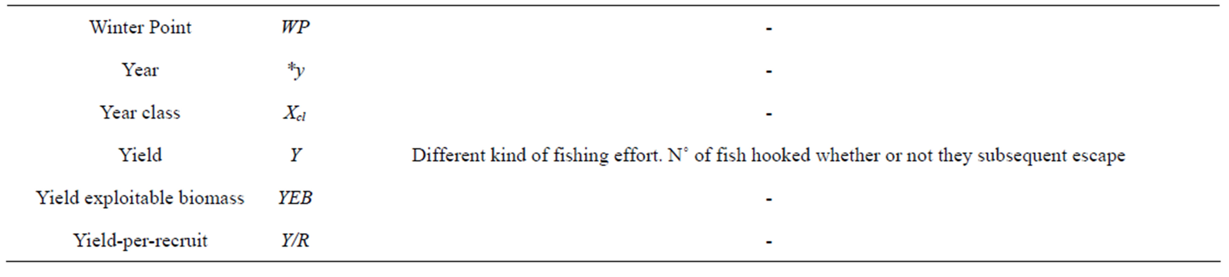
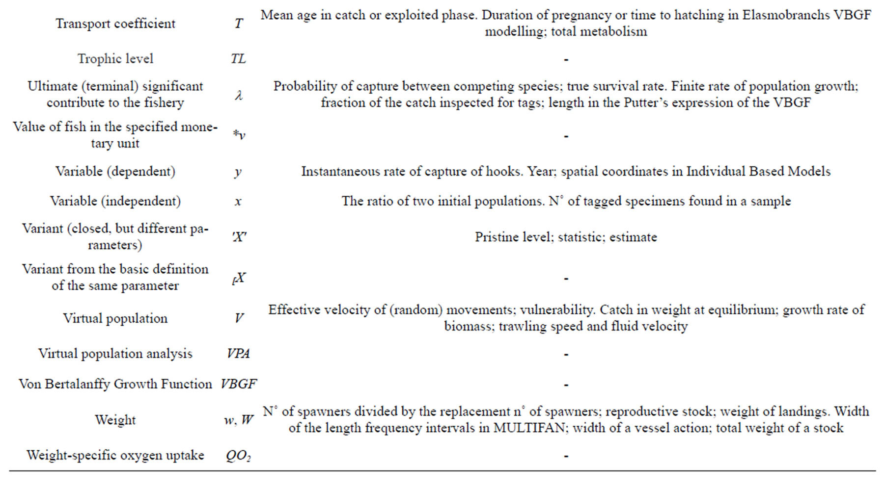
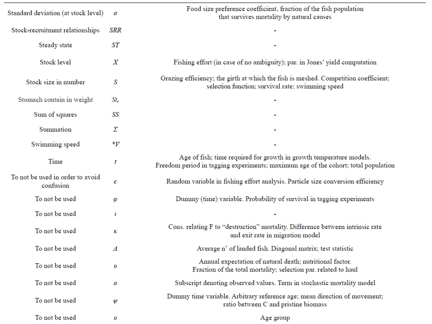
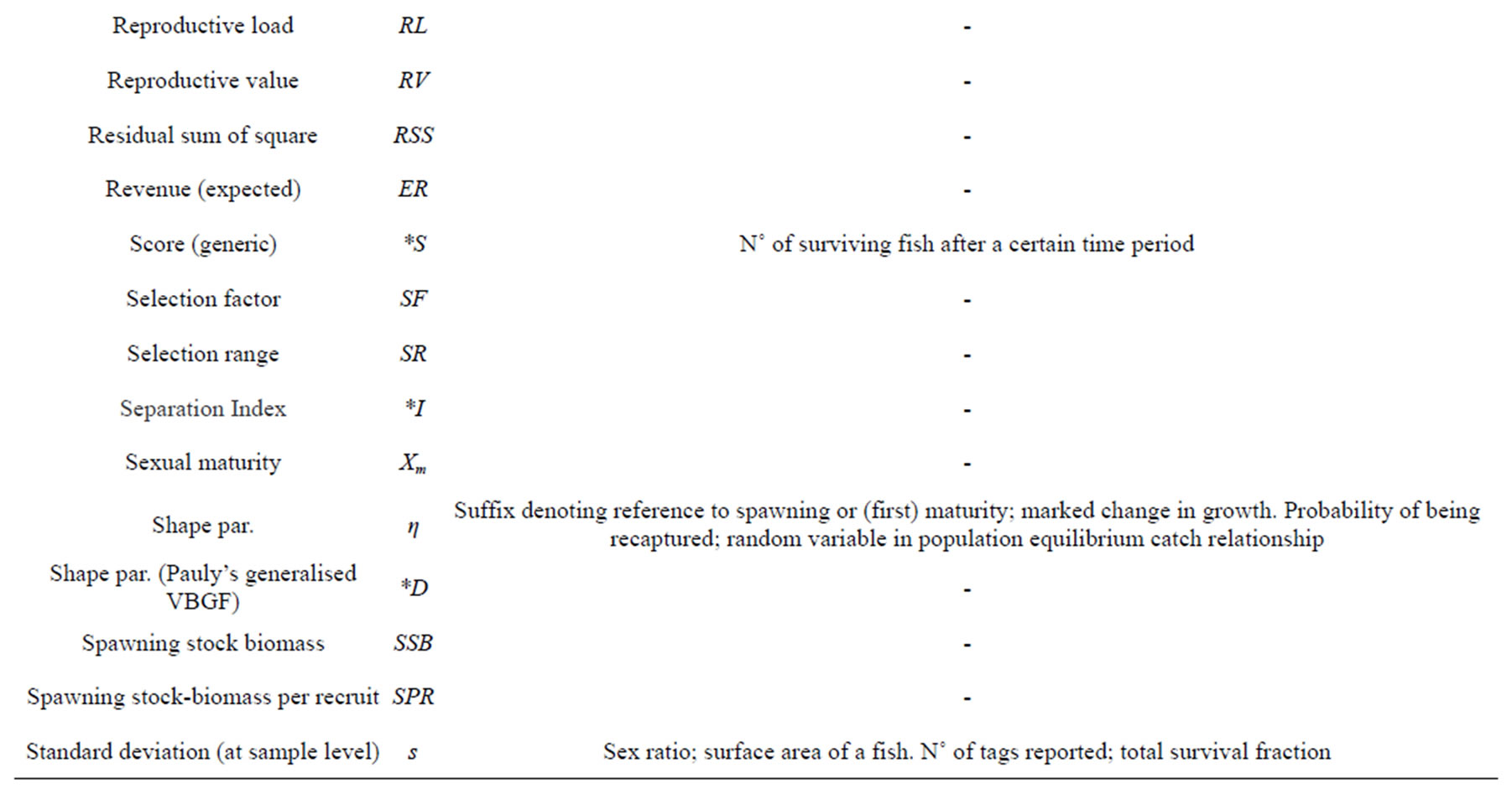
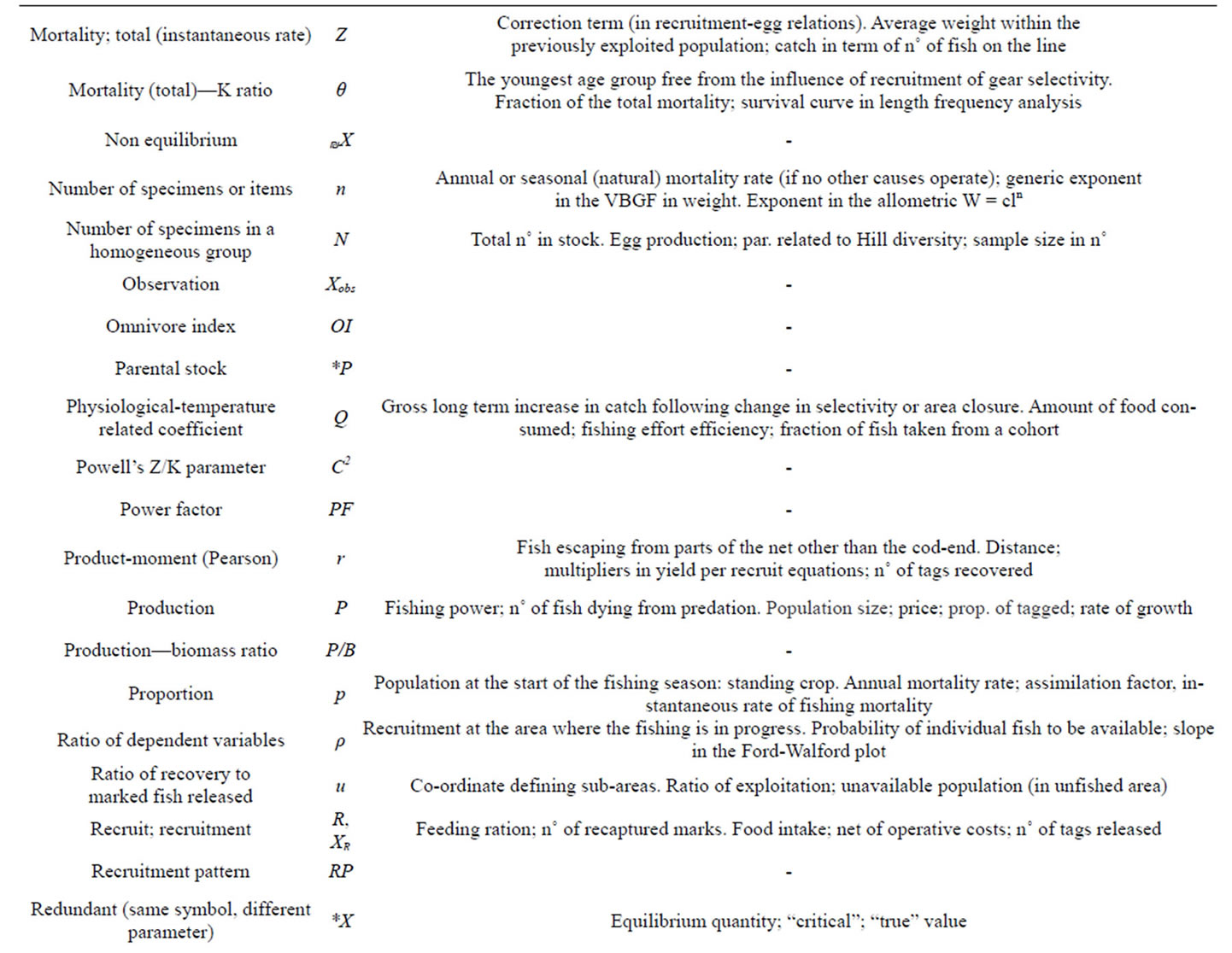
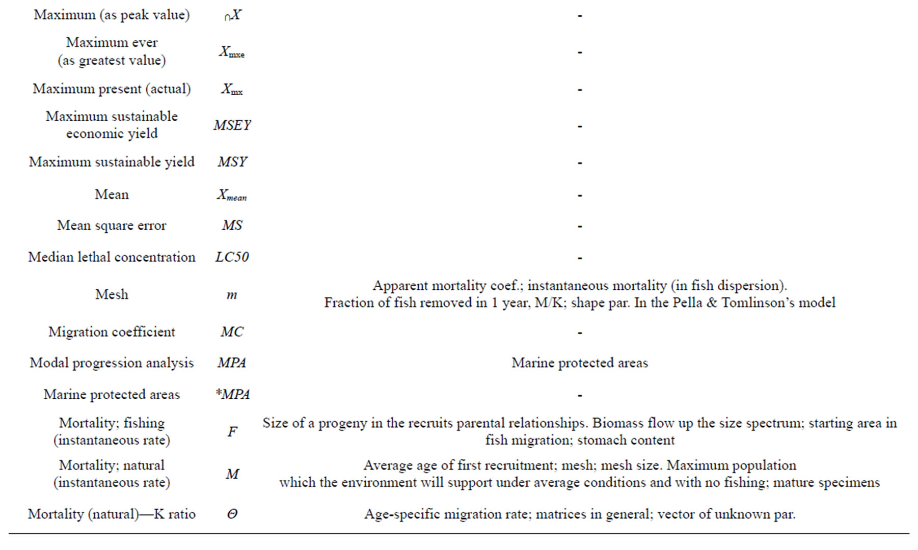
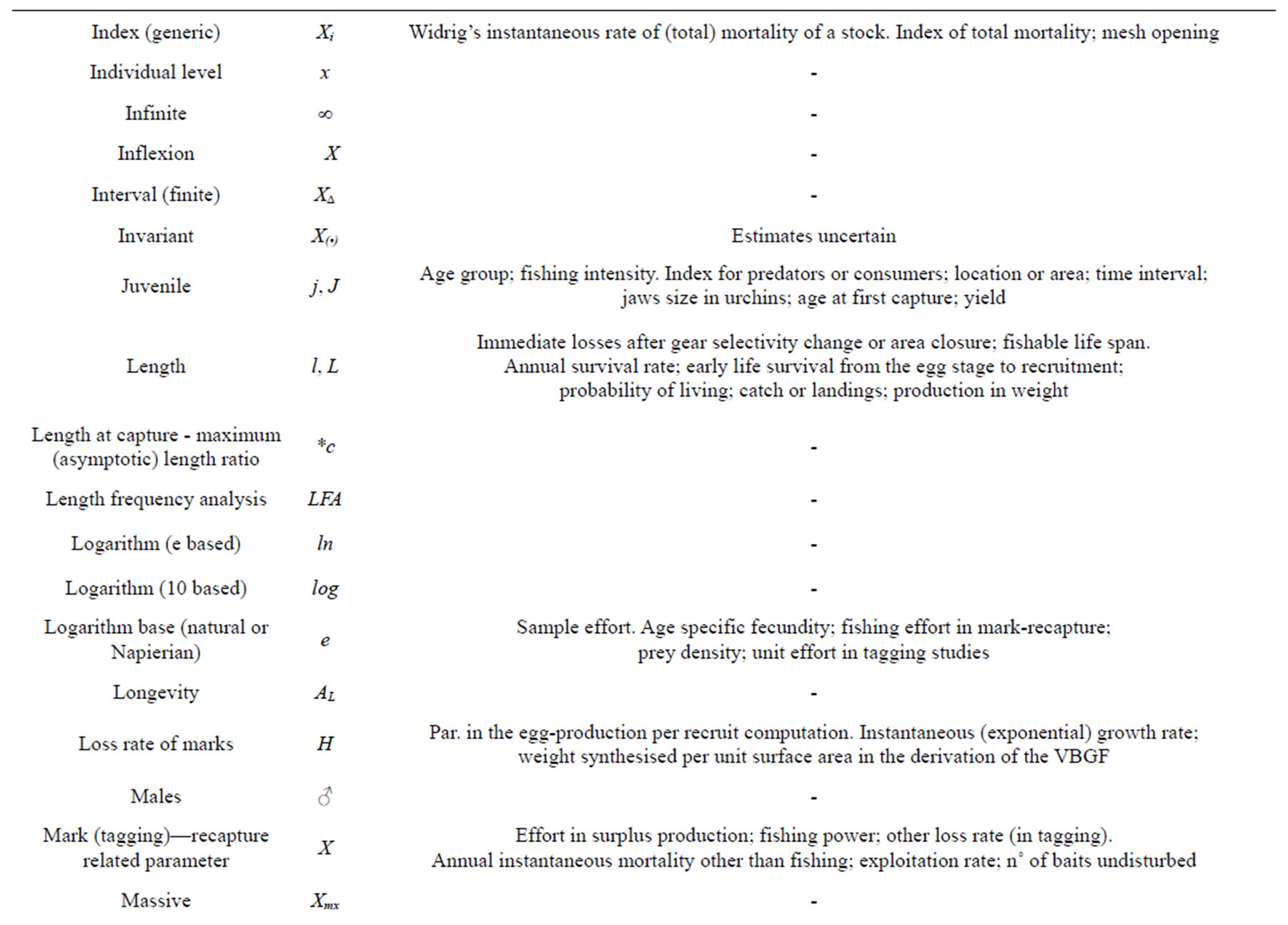
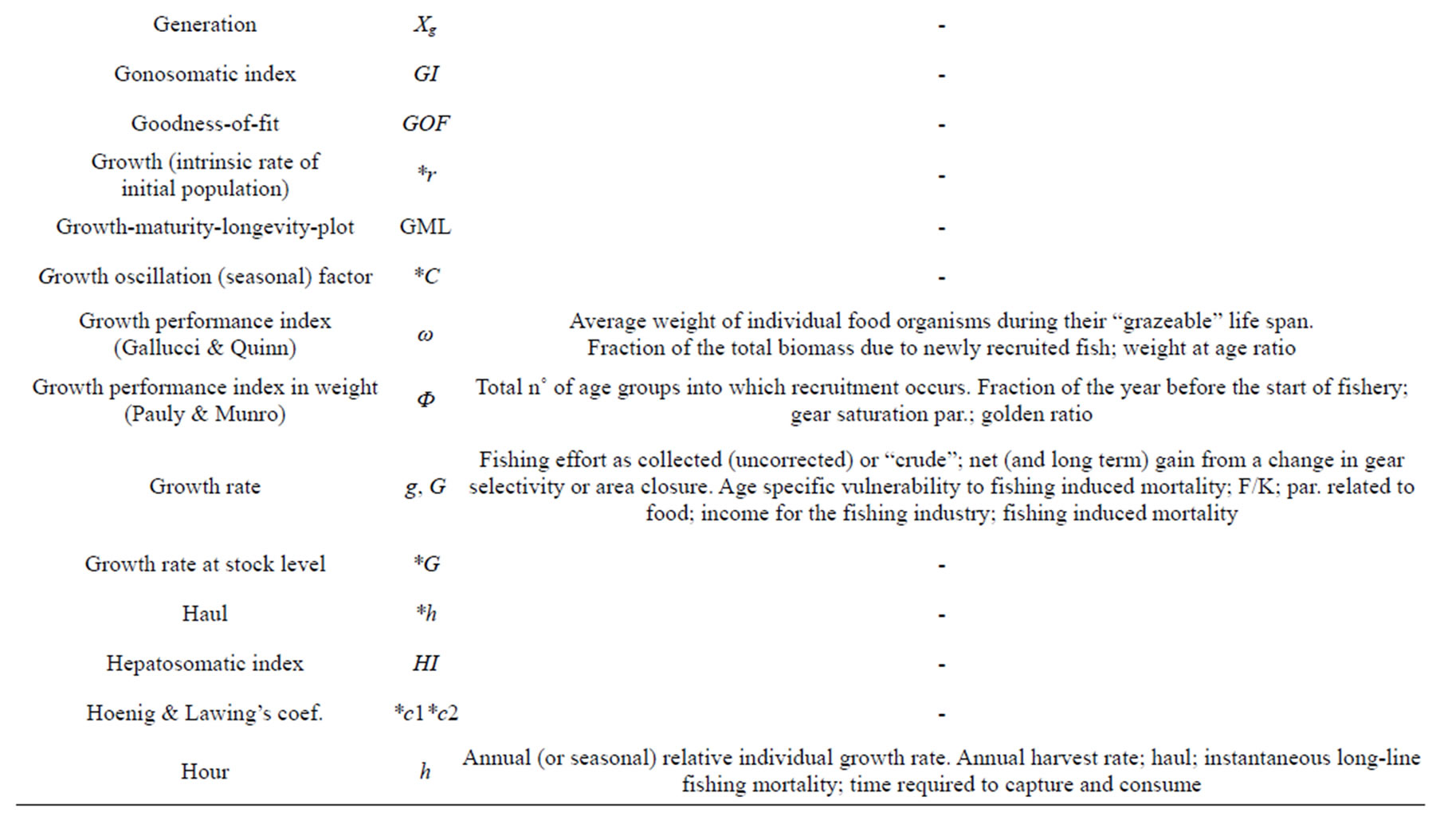
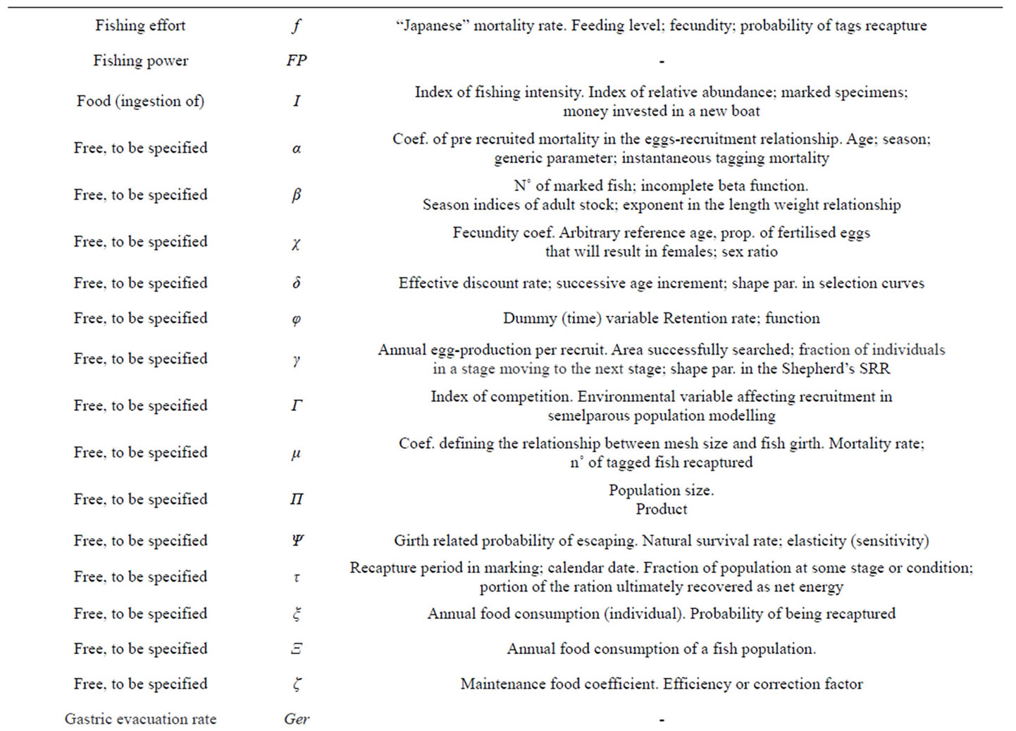
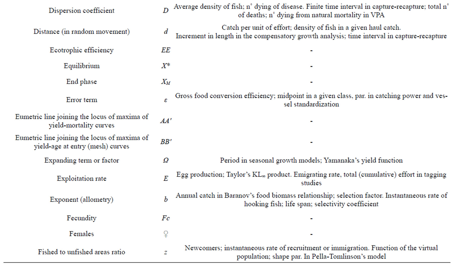
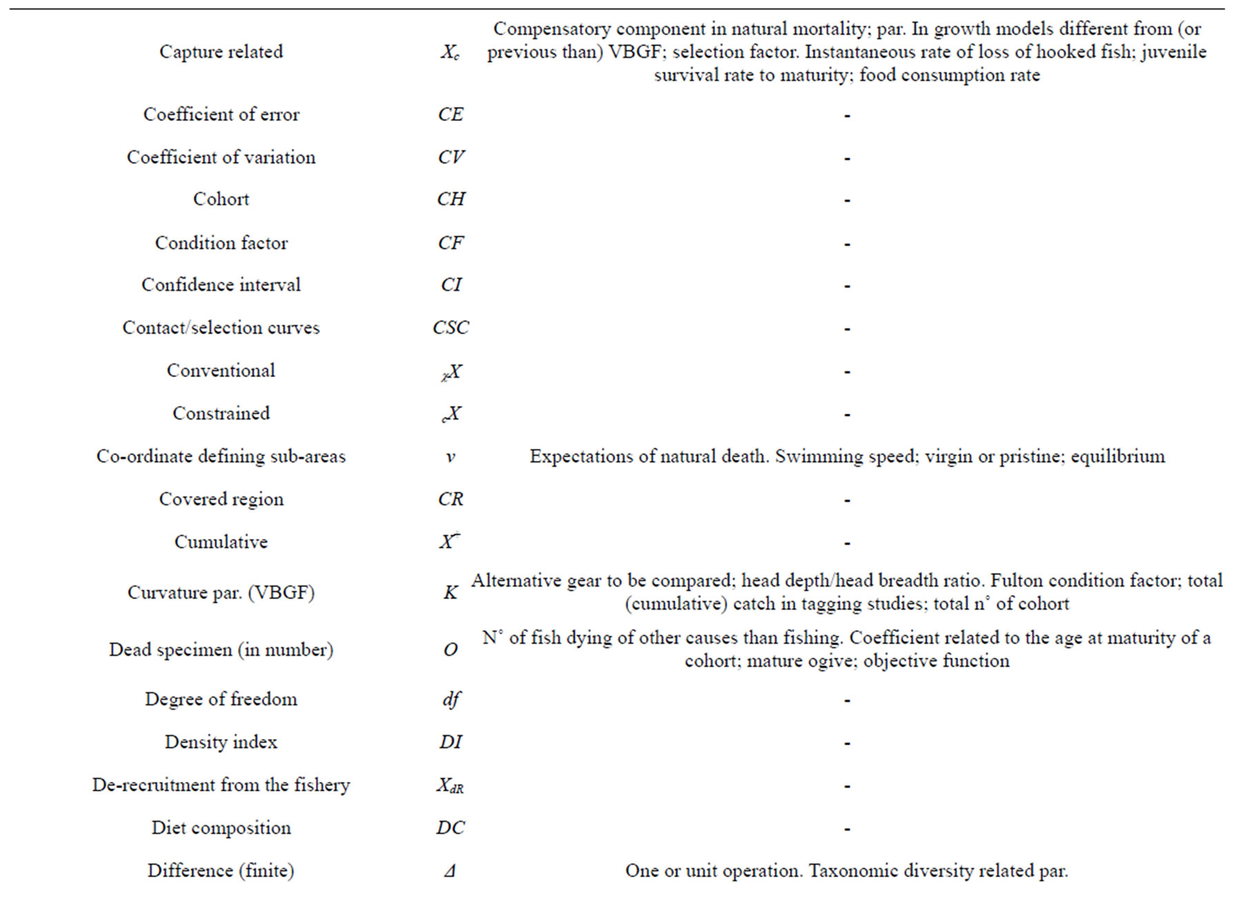
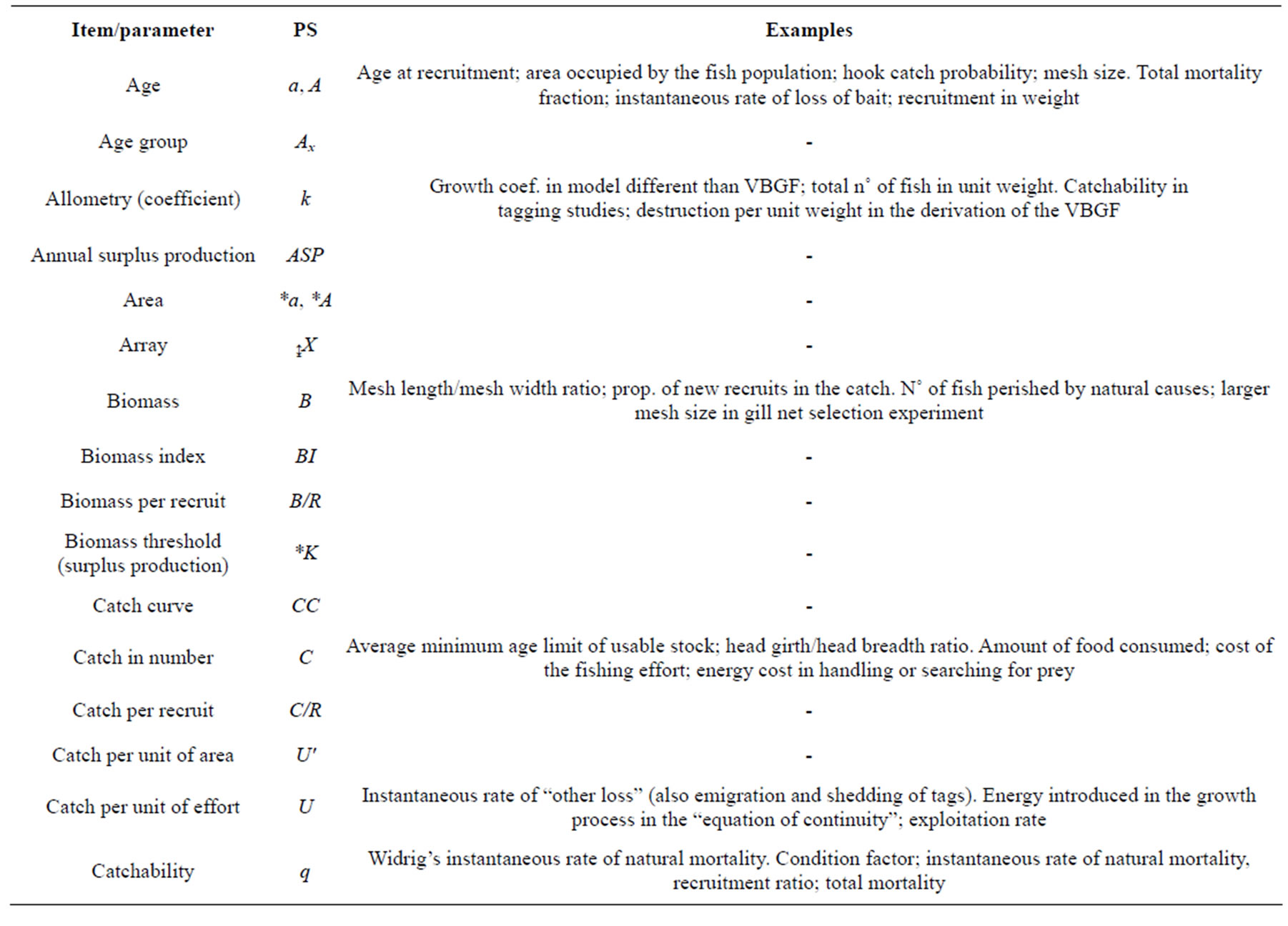
Table 1. Synoptic table of correspondence between item/parameters and symbols proposed (PS) in the present contribute. In the examples column, a selection of other meanings attributed to the given symbol in fishery science are presented (see both the “Milestone” and “Proposed list” sections for abbreviations and other details).
4. ACKNOWLEDGEMENTS
A special thank to Lady Alexis Pacey, Publications Manager of the North Atlantic Fisheries Organisation (NAFO), Dartmouth, NS, who has provided the original historical ICNAF reports and Dr. Adamo Giovanna for her genuine interest in this paper.
REFERENCES
- Cushing, D.H. (1983) Key papers on fish populations. Irl Press, Oxford.
- Smith, T.D. (1988) Stock assessment methods: The first fifty years. In: Gulland, J.A., Ed., Fish Population Dynamics: The Implications for Management, John Wiley and Sons Ltd., Chichester, 1-33.
- Saetersdal, G. (1989) Fish resources research and fishery management: A review of nearly a century of experience in the Northeast Atlantic and some recent global perspectives. Journal du Conseil International pour l’Exploration de la Mer, 46, 5-15.
- Angelini, R. and Moloney, C.L. (2007) Fisheries, ecology and modelling: An historical perspective. Pan-American Journal of Aquatic Sciences, 2, 75-85.
- Beverton, R.J.H. and Holt, S.J. (1956) A review of methods for estimating mortality rates in exploited fish populations, with special reference to sources of bias in catch sampling. Rapports et Procès-Verbaux des RèunI ons Commission Internationale pour l’Exploration Scientifique de la Mer Méditerranée, 140, 67-83.
- Beverton, R.J.H. and Holt, S.J. (1957) On the dynamics of exploited fish populations. Ministry of Agriculture, Fisheries and Food, Lowestoft.
- Beverton, R.J.H. and Holt, S.J. (1959) A review of the lifespans and mortality rates of fishes in nature, and their relation to growth and other physiological characteristics. In: Wolstenholme, C.E.W. and O’Connor, M., Eds., Ciba Foundation Colloquia on Ageing, J and A Churchill Ltd., London, 142-179.
- Gulland, J.A. (1955) On the estimation of growth and mortality in commercial fish population. Fishery Investigations, 18, 46.
- Gulland, J.A. (1956) The study of fish populations by the analysis of commercial catches: A statistical review. Rapports Conseil Internationale pour l’Exploration Scientifique de la Mer Méditerranée, 140, 21-27.
- Gulland, J.A. (1956) A note on the statistical distribution of trawl catches, in problems and methods of sampling fish populations. Rapports Conseil Internationale pour l’Exploration Scientifique de la Mer Méditerranée, 140, 28-29.
- Gulland, J.A. (1962) The application of mathematical models to fish populations. In: Le Cren, E.D. and Holdgate, M.W., Eds., The Exploitation of Natural Animal Populations, Blackwell Scientific Publications, Oxford, 204-217.
- Ricker, W.E. (1954) Stock and recruitment. Journal of the Fisheries Research Board of Canada, 11, 559-623. doi:10.1139/f54-039
- Ricker, W.E. (1958) Handbook of computations for biological statistics of fish populations. Bulletin of the Fisheries Research Board of Canada, 1-300.
- Gulland, J.A. (1958) Notations in fish population studies. ICNAF Special Publication, 1, 69-70.
- Holt, S.J. (1958) Population dynamics: Devise means of reducing the time required to obtain data necessary for making assessment of stocks, especially those required as the basis for a program of conservation. ICNAF Special Publication, 1, 27-50.
- Holt, S.J., Gulland, J.A., Taylor, C. and Kurita, S. (1959) A standard terminology and notation for fishery dynamics. Journal du Conseil International pour l’Exploration de la Mer, 24, 239-242. doi:10.1093/icesjms/24.2.239
- IDWG-LUP (1994) Terminology for integrated resources planning and management. In: Choudhury, K. and Jansen, L.J.M., Eds., Integrated Resources Planning and Management, Food and Agriculture Organization, Rome.
- Coad, B.W. and McAllister, D.E. (2008) Dictionary of ichthyology. http://www.briancoad.com/dictionary/references.htm
- Garcia, S.M. (2009) Glossary. In: Cochrane, K.L. and Garcia, S.M., Eds., A Fishery Manager’s Guidebook, 2nd Edition, Wiley-Blackwell, Hoboken.
- NOAA (2010) Definition of fisheries technical term. http://www.nefsc.noaa.gov/techniques/tech_terms.html#ai
- Restrepo, V.R. (2000) Glossary of fishery terms. ICCAT Standing Committee on Research and Statistics (SCRS). www.iccat.es
- Lleonart, J. (2010) Draft glossary of scientific terms of interest for the SAC General Fisheries Commission for the Mediterranean. Thirty-fourth Session, Athens, 14-17 April 2010, 1-41.
- FAO (2011) Glossary. www.fao.org/fi/glossary/default.asp
- Gulland, J.A. (1983) Stock assessment: Why? FAO Fisheries Circular, 759.
- Hilborn, R. and Walters, C.J. (1992) Quantitative fisheries stock assessment, choice, dynamics and uncertainty. Chapman and Hall, London. doi:10.1007/978-1-4615-3598-0
- Kesteven, G.L. (1999) Stock assessments and the management of fishing activities. Fisheries Research, 44, 105- 112.
- Musick, J.A. and Bonfil, R. (2005) Management techniques for elasmobranch fisheries. FAO Fisheries Technical Paper, 474, 1-251.
- Huntsman, A.G. (1953) Fishery management and research. Journal du Conseil International pour l’Exploration de la Mer, 14, 44-55.
- ICNAF (1960) The selectivity of fishing gear. Proceedings of the joint scientific meeting of ICNAF, ICES, and FAO on fishing effort, the effect of fishing on resources and the selectivity of fishing gear, Lisbon, 27 May-3 June 1957.
- Gulland, J.A. (1969) Manual of methods for fish stock assessment. Part 1. Fish population analysis. FAO Manual Fisheries Science.
- Clark, S.H. (1979) Application of bottom-trawl survey data to fish stock assessment. Fisheries, 4, 9-15. doi:10.1577/1548-8446(1979)004<0009:AOBSDT>2.0.CO;2
- Caddy, J.F. (2009) Practical issues in choosing a framework for resource assessment and management of Mediterranean and Black Sea fisheries. Mediterranean Marine Science, 10, 83-119. doi:10.12681/mms.124
- Beverton, R.J.H. (1953) Some observations on the principles of fishery regulation. Journal du Conseil Permanent International pour l’Exploration de la Mer, 19, 56- 68.
- Beverton, R.J.H. and Parrish, B.B. (1956) Commercial statistics on fish population studies. Rapports et ProcèsVerbaux des Rèunions Commission Internationale pour l’Exploration Scientifique de la Mer Méditerranée, 140, 58-66.
- Holt, S.J. (1958) The evaluation of fisheries resources by the dynamic analysis of stocks, and notes on the time factors involved. ICNAF Special Publication, 1, 77-95.
- Holt, S.J. (1963) A method for determining gear selectivity and its application. ICNAF Special Publication, 5, 106-115.
- Holt, S.J. (1965) A note on the relation between the mortality rate and the duration of life in an exploited fish population. ICNAF Research Bulletin, 2, 73-75.
- Gulland, J.A. (1961) The estimation of the effect on catches of changes in gear selectivity. Journal du Conseil International pour l’Exploration de la Mer, 26, 204-214.
- Gulland, J.A. (1964) A note on the interim effects on catches of changes in gear selectivity. Journal du Conseil International pour l’Exploration de la Mer, 29, 61-64.
- Gulland, J.A. (1964) Catch per unit effort as a measure of abundance. Rapports et Procès-Verbaux des Rèunions Commission Internationale pour l’Exploration Scientifique de la Mer Méditerranée, 155, 8-14.
- Gulland, J.A. (1964) Variations in selection factors and mesh differentials. Journal du Conseil International pour l’Exploration de la Mer, 29, 158-165.
- Gulland, J.A. (1967) Further notes on the effect of possible regulatory measures on catches of Greenland cod. ICNAF Redbook, Part III: 34-47.
- Gulland, J.A. (1977) Fish population dynamics: The implications for management. Wiley Interscience, New York.
- Gulland, J.A. (1983) Fish stock assessment: A manual of basic methods. Wiley Interscience, Chichester.
- Gulland, J.A. (1987) Natural mortality and size. Marine Ecology Progress Series, 39, 197-199.
- Gulland, J.A. and Holt, S.L. (1959) Estimation of growth parameters for data at unequal time intervals. Journal du Conseil International pour l’Exploration de la Mer, 25, 47-49.
- ICNAF (1958) Some problems for biological fishery survey, and techniques for their solution. ICNAF Research Bulletin, 1.
- ICNAF (1962) Report of the working group of scientists on fishery assessment in relation to regulation problems. In: Beverton, R.J.H. and Hodder, V.M., Eds., A Proceedings of the International Commission of the NW Atlantic Fisheries, 11, 1-81.
- ICNAF (1963) The selectivity of fishing gear. ICNAF Special Publication, 5.
- ICNAF (1967) Selected papers from the 1966 annual meeting. Redbook Part III, Dartmouth.
- Kesteven, G.K. and Holt, S.J. (1955) A note on the fisheries resources of the north west Atlantic. FAO Fisheries Paper, 7, 1-12.
- Ricker, W.E. (1940) Relation of “catch per unit effort” to abundance and rate of exploitation. Journal of the Fisheries Research Board of Canada, 5, 43-70. doi:10.1139/f40-008
- Ricker, W.E. (1958) Production, reproduction and yield. Veroffentlichungen Limnologie, 13, 84-100.
- Ricker, W.E. (1963) Big effects from small causes: Two examples from fish population dynamics. Journal of the Fisheries Research Board of Canada, 20, 257-264. doi:10.1139/f63-022
- Ricker, W.E. (1973) Critical statistics from two reproductive curves. Rapports et Procès-Verbaux des Rèunions Commission Internationale pour l’Exploration Scientifique de la Mer Méditerranée, 164, 333-340.
- Ricker, W.E. (1975) Computation and interpretation of biological statistics of fish population. Bulletin of the Fisheries Research Board of Canada, 191.
- Ricker, W.E. (1977) The historical development. In: Gulland, J.A., Ed., Fish Population Dynamics: The Implications for Management, Wiley Interscience, New York, 1- 26.
- Ricker, W.E. (1979) Growth rates and models. In: Hoar, W.S., Randall, D.J. and Brett, J.R., Eds., Fish Physiology, III, Bioenergetics and Growth, Academic Press, New York, 677‑743.
- William, E. and Ricker, R.E. (1948) Computation of fish production. A Symposium on Fish Populations. Proceedings of the Meeting held at the Royal Ontario Museum of Zoology, Toronto, 10-11 January 1947, 173-211.
- Liungman, C.G. (2004) Symbols: Encyclopaedia of western signs and ideograms. 3rd Edition, HME Publishing, Stockholm.
- Gjøsæter, H., Bogstad, B. and Tjelmeland, S. (2002) Assessment methodology for Barents Sea capelin, Mallotus villosus (Müller). ICES Journal of Marine Sciences, 59, 1086-1095. doi:10.1006/jmsc.2002.1238
- Taylor, C.C. (1958) Cod growth and temperature. Journal du Conseil International pour l’Exploration de la Mer, 23, 366-370.
- Marutani, T. (2008) On the optimal path in the dynamic pool model for a fishery. Reviews in Fish Biology and Fisheries, 18, 133-141. doi:10.1007/s11160-007-9065-7
- Schnute, J. (1987) A general fishery model for a sizestructured fish population. Canadian Journal of Fisheries and Aquatic Sciences, 44, 924-940. doi:10.1139/f87-111
- Quinn, T.J. II and Deriso, R.B. (1999) Quantitative fish dynamics. Oxford University Press, Oxford.
- Gayanilo Jr., F.C., Sparre, P. and Pauly, D. (2005) FAOICLARM stock assessment tools II (FiSAT II). User’s guide. FAO Computerized Information Series (Fisheries), 8.
- Christie, W.J. and Spangler, G.R. (1987) The international symposium on stock assessment and yield prediction. Canadian Journal of Fisheries and Aquatic Sciences, 44, 501.
- Jennings, S., Kaiser, M.J. and Reynolds, J.D. (2001) Marine fisheries ecology. Blackwell Science, Oxford.
- Widrig, T.M. (1954) Method of estimating fish populations with application to Pacific sardine. Fishery Bulletin of the United States of America, 56, 141-166.
- Hart, P.J.B. and Reynolds. J.D. (2002) Handbook of fish biology and fisheries (1-2). Blackwell Science Ltd., Oxford.
- Pauly, D. (1984) Fish populations dynamics in tropical waters. International Center for Living Aquatic Resources Management, Manila.
- Pauly, D. and Morgan, G.R. (1987) Length-based methods in fisheries research. International Center for Living Aquatic Resources Management, Manila.
- Millar, R.B. and Fryer, R.J. (1999) Estimating size-selection curves of trawls, traps, gillnets, and hooks. Reviews in Fish Biology and Fisheries, 9, 89-116. doi:10.1023/A:1008838220001
- Sparre, P. and Venema, S.C. (1998) Introduction to tropical fish stock assessment, Part I: Manual. FAO Fisheries Technical Paper, 306, 1.
- Chen, S. and Watanabe, S. (1989) Age dependence of natural mortality coefficient in fish population dynamics. Nippon Suisan Gakkaishi, 55, 205-208. doi:10.2331/suisan.55.205
- Laurec, A. and Le Guen, J.C. (1981) Dynamique des population marines exploitées. Publication CNEXO Rapport Scientific et Technologic, 45, 1-111.
- Kutty, M.K. and Qasim, S.Z. (1968) The estimation of optimum age of exploitation and potential yield in fish populations. Journal du Conseil International pour l’Exploration de la Mer, 32, 249-255. doi:10.1093/icesjms/32.2.249
- Hjort, J., Jahn, G. and Ottestad, P. (1933) The optimum catch. Hvalradets Skrifter, 7, 92-107.
- May, R.C. (1974) Larval mortality in marine fishes and the critical period concept. In: Blaxter, J.H.S., Ed., The Early Life History of Fish, Spring-Verlag, Berlin, 3-19. doi:10.1007/978-3-642-65852-5_1
- Smith, P.E. (1985) Year-class strength and survival of 0 group clupeoids. Canadian Journal of Fisheries and Aquatic Sciences, 2, 69-82.
- [82] Bethke, E. (2004) A simple general approach to codend selectivity of trawls and its application to the data of Fiorentino et al. (1998) for Hake (Merluccius merluccius). Fisheries Research, 70, 113-119. doi:10.1016/j.fishres.2004.05.012
- Walters, C., Christensen, V. and Pauly, D. (1997) Structuring dynamic models of exploited ecosystems from trophic mass-balance assessments. Reviews in Fish Biology and Fisheries, 7, 139-172. doi:10.1023/A:1018479526149
- Mertz, G. and Myers, R.A. (1998) A simplified formulation for fish production. Canadian Journal of Fisheries and Aquatic Sciences, 55, 478-484. doi:10.1139/f97-216
- Schnute, J.T. and Richards, L.J. (1998) Analytical models for fishery reference points. Canadian Journal of Fisheries and Aquatic Sciences, 55, 515-528. doi:10.1139/f97-212
- Pope, J.G. (1977) Estimation of fishing mortality, its precision and implications for the management of fisheries. In: Steele, J.H., Ed., Fisheries Mathematics, Academic Press, London, 63-76.
- Megrey, B.A. (1989) Review and comparison of agestructured stock assessment models from theoretical and applied points of view. American Fisheries Society Symposium, 6, 8-48.
- Charnov, E.L. (1993) Life history invariants. Some explorations of symmetry in evolutionary ecology. Oxford University Press, Oxford.
- Russell, E.S. (1931) Some theoretical consideration on the overfishing problem. Journal du Conseil International pour l’Exploration de la Mer, 6, 3-20.
- Tester, A.I. (1955) Estimation of recruitment and natural mortality rate from age-composition and catch data in British Columbia Herring population. Journal of the Fisheries Research Board of Canada, 12, 649-641. doi:10.1139/f55-035
- Murphy, G.I. (1960) Estimating abundance from long-line catches. Journal of the Fisheries Research Board of Canada, 17, 33-40. doi:10.1139/f60-003
- Taylor, C.C. (1962) Growth equations with metabolic parameters. Journal du Conseil International pour l’Exploration de la Mer, 27, 270-286.
- Jones, R. (1977) Tagging: Theoretical methods and practical difficulties. In: Gulland, J.A., Ed., Fish Population Dynamics: The Implications for Management, Wiley Interscience, New York, 46-66.
- Baker, T.T., Lafferty, R. and Quinn II, T.J. (1991) A general growth model for mark-recapture data. Fisheries Research, 1, 257-281. doi:10.1016/0165-7836(91)90005-Z
- Alverson, D.L. and Pereyra, W.T. (1969) Demersal fish explorations in the north-eastern Pacific Ocean—An evaluation of exploratory fishing methods and analytical approaches to stock size and yield forecasts. Journal of the Fisheries Research Board of Canada, 26, 1985-2001. doi:10.1139/f69-188
- Herrington, W.C. (1948) Limiting factors for fish populations. Some theories and an example. A Symposium on Fish Populations. Proceedings of the Meeting Held at the Royal Ontario Museum of Zoology, Toronto, 10-11 January 1947, 229-283.
- Schaefer, M.B. (1957) Some considerations of population dynamics and economics in relation to the management of commercial marine fisheries. Journal of the Fisheries Research Board of Canada, 14, 669-681. doi:10.1139/f57-025
- Paulik, G.J. (1961) Detection of incomplete reporting of tags. Journal of the Fisheries Research Board of Canada, 18, 817-832. doi:10.1139/f57-025
- Paloheimo, J.E. and Dickie, L.M. (1966) Food and growth of fishes. II. Effects of food and temperature on the relation between metabolism and body weight. Journal of the Fisheries Research Board of Canada, 23, 869- 908. doi:10.1139/f66-077
- Jones, R. and Johnston, C. (1977). Growth, reproduction and mortality in gadoid fish species. In: Steele, J.H., Ed., Fisheries Mathematics, Academic Press, London, 37-62.
- Charnov, E.L., Berrigan, D. and Shine, R. (1993) The M/K ratio is the same for fish and reptiles. American Naturalist, 142, 707-711. doi:10.1086/285565
- Francis, R.I.C.C. (1988) Are growth parameters estimated from tagging and age-length data comparable? Canadian Journal of Fisheries and Aquatic Sciences, 45, 936-942. doi:10.1139/f88-115
- Fournier, D.A., Sibert, J.R., Majkowski, J. and Hampton, J. (1990) MULTIFAN, a likelihood‑based method for estimating growth parameters and age composition from multiple length frequency data sets illustrated using data for Southern bluefin tuna (T. maccoyii). Canadian Journal of Fisheries and Aquatic Sciences, 47, 301‑317. doi:10.1139/f90-032
- Yamakawa, T. and Matsuda, H. (1997) Improved bêlehrádek’s equation for a comprehensive description of the relationship between environmental factors and metabolic rates. Fisheries Science, 63, 725-773.
- Cadima, E.L. (2003) Fish stock assessment manual. FAO Fisheries Technical Paper, 393.
- Graham, M. (1935) Modern theory of exploiting a fishery, and application to North Sea trawling. Journal du Conseil International pour l’Exploration de la Mer, 10, 264-274.
- Foster, J.J., Ferro, R.S.T. and Reid, A.J. (1977) Analytic approaches in fishing technology. In: Steele, J.H., Ed., Fisheries Mathematics, Academic Press, London, 99-116.
- Brethes, J.C. and O’Boyle, R.N. (1990) Methodes d’evaluation des stocks halieutiques. Centre International d’Exploitation des Oceans, Halifax, 933.
- Gayanilo Jr., F.C. and Pauly, D. (1997) FAO-ICLARM fish stock assessment (FiSAT) reference manual. FAO Computerized Information Series (Fisheries), 8, 2.
- Froese, R. and Pauly, D. (1998) FishBase 98: Concepts, design and data sources. International Center for Living Aquatic Resources Management, Manila.
- Caddy, J.F. (1983) The cephalopods: Factors relevant to their population dynamics and to the assessment and management of stocks. FAO Fisheries Technical Paper, 231, 416-452.
- Alverson, D.L. and Carney, M.J. (1975) A graphic review of the growth and decay of population cohorts. Journal du Conseil International pour l’Exploration de la Mer, 36, 133-143.
- Hoenig, J.M. (1983) Empirical use of longevity data to estimate mortality rates. Fishery Bulletin of the United States of America, 82, 898-902.
- Beverton, R.J.H. (1992) Patterns of reproductive strategy parameters in some marine teleost fishes. Journal of Fish Biology, 41, 137-160.
- Hewitt, D.A. and Hoenig, J.M. (2005) Comparison of two approaches for estimating natural mortality based on longevity. Fishery Bulletin of the United States of America, 103, 433-437.
- Rosenberg, A.A. and Beddington, J.R. (1988) Lengthbased methods of fish stock assessment. In: Gulland, J.A., Ed., Fish Population Dynamics, John Wiley and Sons, Chichester, 83-103.
- Froese, R. (2006) Cube law, condition factor and weightlength relationships: History, meta-analysis and recommendations. Journal of Applied Ichthyology, 22, 241-253. doi:10.1111/j.1439-0426.2006.00805.x
- Hoggarth, D.D., Abeyasekera, S., Arthur, R.I., Beddington, J.R., et al. (2006) Stock assessment for fishery management—A framework guide to the stock assessment tools of the Fisheries Management Science Programme (FMSP). FAO Fisheries Technical Paper, 487.
- Allen, K.R. (1953) A method for computing the optimum size limit for a fishery. Nature London, 172, 210. doi:10.1038/172210a0
- Allen, K.R. (1967) Some quick methods for estimating the effect on catch of changes in the size limit. Journal du Conseil International pour l’Exploration de la Mer, 31, 111-126.
- Tanaka, S. (1962) The effect of reduction of fishing effort on Yield. Journal of the Fisheries Research Board of Canada, 19, 521-529. doi:10.1139/f62-035
- Ebert, T.A. (1982) Longevity, life history and relative body wall size in sea urchins. Ecological Monographs, 52, 353-394. doi:10.2307/2937351
- Chapman, D.G. (1961) Statistical problems in dynamics of exploited fisheries populations. In: Neyman, J., Ed., Proceedings of the Fourth Berkeley Symposium on Mathematical Statistics and Probability, Vol. 4. University of California Press, Berkeley, 153-168.
- Ivlev, V.S. (1961) Mathematical analysis of the population dynamics of fish. Israel Program for scientific translation (form the Russian, original published in 1959).
- Caddy, J.F. (1996) Modelling natural mortality with age in short-lived invertebrate populations: Definition of a strategy of gnomonic time division. Aquatic Living Resources, 9, 197-207. doi:10.1051/alr:1996023
- Jensen, A.J.C. (1949) The relation between size of mesh and length of fish released. Rapports et Procès-Verbaux des Rèunions Commission Internationale pour l’Exploration Scientifique de la Mer Méditerranée, 125, 65-69.
- Pope, J.A., Margetts, A.R., Hamley, J.M. and Akyuz, E.F. (1983) Manual of methods for fish stock assessment; part 3: Selectivity of fishing gear. FAO Fisheries Technical Paper, 41, 1-56.
- Bishop, Y.M.M. (1959) Errors in estimates of mortality obtained from virtual populations. Journal of the Fisheries Research Board of Canada, 16, 73-90. doi:10.1139/f59-009
- Die, D.J. and Caddy, J.F. (1997) Sustainable yield indicators from biomass: Are there appropriate reference points for use in tropical fisheries? Fisheries Research, 32, 69-79. doi:10.1016/S0165-7836(97)00029-5
- Schaefer, M.B. (1957) A study of the dynamics of the fishery for yellowfin tuna in the eastern tropical Pacific Ocean. Bulletin of the Inter-American Tropical Tuna Commission, 2, 247-285.
- Jones, R. (1956) The analyses of trawl haul statistics with particular reference to the estimation of survival rates. Rapports et Procès-Verbaux des Rèunions Commission Internationale pour l’Exploration Scientifique de la Mer Méditerranée, 140, 30-39.
- Cushing, D.H. and Horwood, J.W. (1977) Development of a model of stock and recruitment. In: Steele, J.-H., Ed., Fisheries Mathematics, Academic Press, London, 21-35.
- Carrothers, P.J.G. (1980) Estimation of trawl door spread from wing spread. Journal of Northwest Atlantic Fishery Science, 1, 81-90.
- Doubleday, W.G. and Rivard, D. (1981) Canadian special publication of fisheries and aquatic sciences. Botton Trawl Surveys, 58.
- Campbell, N.A. and Phillips, B.F. (1972) The von Bertalanffy growth curve and its application to capture-recapture data in fisheries biology. Journal du Conseil International pour l’Exploration de la Mer, 34, 295-299.
- Katsanevakis, S. (2006) Modelling fish growth: Model selection, multi-model inference and model selection uncertainty. Fisheries Research, 81, 229-235. doi:10.1016/j.fishres.2006.07.002
- Nikolsky, G.V. (1963) The ecology of fishes. Academic Press Inc., London.
- Ramm, D.C. and Xiao, Y. (1995) Herding in groundfish and effective path width of trawls. Fisheries Research, 24, 243-259. doi:10.1016/0165-7836(95)00373-I
- Pauly, D. (1981) The relationships between gill surface area and growth performance in fish; a generalisation of von Bertalanffy’s theory of growth. Meeresforschung, 28, 251-282.
- De Lury, D.B. (1961) On the planning of experiments for the estimation of fish populations. Journal of the Fisheries Research Board of Canada, 8, 281-307.
- Andersen, K.P. and Ursin, E. (1977) A multispecies extension to the Beverton and Holt theory of fishing, with accounts of phosphorus circulation and primary production. Meddelelser fra Danmarks Fiskeri-Og Havundersogelser, 7, 319-435.
- Nicholson, M.D. and Pope, J.A. (1977) The estimation of mortality from capture-recapture experiments. In: Steele, J.H., Ed., Fisheries Mathematics, Academic Press, London, 77-85.
- Sissenwine, M.P., Fogarty, M.I. and Overholtz, W.J. (1988) Some fisheries management implications of recruitment variability. In: Gulland, J.A., Ed., Fish Population Dynamics, John Wiley & Sons, New York, 129-152.
- Ware, D.M. (1975) Growth, metabolism, and optimal swimming speed of a pelagic fish. Journal of the Fisheries Research Board of Canada, 32, 33-41. doi:10.1139/f75-005
- Rothschild, B.J. and Suda, A. (1977) Population dynamics of tuna. In: Gulland, J.A., Ed., Fish Population Dynamics, John Wiley and Sons, New York, 309-334.
- Cushing, D.H. (1981) Fisheries biology: A study in population dynamics. University of Wisconsin Press, Madison.
- Harden, J.F.R. (1977) Performance and behaviour on migration. In: Steele, J.H., Ed., Fisheries Mathematics, Academic Press, London, 145-170.
- Barkley, R.A. (1964) The theoretical effectiveness of towed-net samplers as related to sample size and swimming speed of organisms. Journal du Conseil Permanent International pour l’Exploration de la Mer, 24, 146-157.
- Davis, F.M. (1934) Mesh experiments with trawls 1928- 1933. Fishery Investigation, 14, 1-56.
- Houghton, R.G. (1977) The fishing power of trawlers in the western English Channel between 1965 and 1968. Journal du Conseil International pour l’Exploration de la Mer, 37, 130-136. doi:10.1093/icesjms/37.2.130
- Treschev, A.I. (1978) Application of the fished volume method for measuring fishing effort. ICES Cooperative Research Report, 79, 1-55.
- Anganuzzi, A., Hilborn, R. and Skalski, J.R. (1994) Estimation of size selectivity and movement rates from mark-recovery data. Canadian Journal of Fisheries and Aquatic Sciences, 51, 734-742. doi:10.1139/f94-073
- Stamps, J.A., Mangel, M. and Phillips, J.A. (1998) A new look at relationships between size at maturity and asymptotic size. American Naturalist, 152, 470-479.
- Beyer, J.E., Kirchner, C.H. and Holtzhausen, J.A. (1999) A method to determine size-specific natural mortality applied to westcoast steenbras (Lithognathus aureti) in Namibia. Fisheries Research, 41, 133-155. doi:10.1016/S0165-7836(99)00011-9
- Southward, G.M. and Chapman, D.G. (1965) Utilization of Pacific halibut stocks: Study of Bertalanffy’s growth equation. International Pacific Halibut Commission Scientific Report, 39, 1-33.
- Cortés, E. (2000) Life history patterns and correlations in sharks. Review in Fisheries Science, 8, 299-344.
- Rothschild, B.J. (1977) Fishing effort. In: Gulland, J.A., Ed., Fish Population Dynamics, John Wiley and Sons, New York, 96-115.
- Cushing, D.H. (1988) The study of stock and recruitment. In: Gulland, J.A., Ed., Fish Population Dynamics, John Wiley and Sons, Chichester, pp. 105-128.
- Tomlinson, P.K. and Abramson, N.J. (1961) Fitting a von Bertalanffy growth curve by the least squares. California Fish and Game Fish Bulletin, 116, 1-69.
- Holden, M.J. (1977) Elasmobranchs. In: Gulland, J.A., Ed., Fish Population Dynamics, John Wiley & Sons, Chichester, 187-215.
- Francis, R.I.C.C. (1995) The analysis of otolith data—A mathematician’s perspective (What precisely is your model?). In: Secor, D.H., Dean, J.M. and Campana, S.E., Eds., Recent Developments in Fish Otolith Research, University of South Carolina Press, Columbia.
- Lockwood, S.J. (1974) The use of the von Bertalanffy growth equation to describe the seasonal growth of fish. Journal du Conseil International pour l’Exploration de la Mer, 35, 175-179.
- MacDonald, P.D.M. and Pitcher, T.J. (1979) Age-groups from size-frequency data: A versatile and efficient method of analysing distribution mixtures. Journal of the Fisheries Research Board of Canada, 36, 987-1001. doi:10.1139/f79-137
- Caddy, J.F. (1991) Death rates and time intervals: Is there an alternative to the constant natural mortality axiom? Reviews in Fish Biology and Fisheries, 11, 109‑118. doi:10.1007/BF00157581
- Roff, D.A. (1984) The evolution of life history parameters in teleosts. Canadian Journal of Fisheries and Aquatic Sciences, 41, 989-1000. doi:10.1139/f84-114
- Beverton, R.J.H. and Iles, T.C. (1992) Mortality rates of 0-group plaice (Pleuronectes platessa L.), dab (Limanda limanda L.) and turbot (Scophthalmus maximus L.) in European waters: II. Comparison of mortality rates and construction of life-table for 0-group plaice. Netherland Journal of Sea Research, 29, 49-59. doi:10.1016/0077-7579(92)90007-2
- Gallucci, V.F. and Quinn T.J. II (1979) Reparameterizing, fitting, and testing a simple growth model. Transactions of the American Fisheries Society, 108, 14-25. doi:10.1577/1548-8659(1979)108<14:RFATAS>2.0.CO;2
- Allen, K.R. (1971) Relation between production and biomass. Journal of the Fisheries Research Board of Canada, 28, 1573-1581.
- Robson, D.S. (1966) Estimation of the relative fishing power of individual ships. ICNAF Research Bulletin, 3, 5- 14.
- Arreguín-Sánchez, F. (1996) Catchability: A key parameter for fish stock assessment. Reviews in Fish Biology and Fisheries, 6, 221-242. doi:10.1007/BF00182344
- Myers, R.A. and Doyle, R.W. (1983) Predicting natural mortality rates and reproduction—Mortality trade-offs from fish life history data. Canadian Journal of Fisheries and Aquatic Sciences, 40, 612-620. doi:10.1139/f83-080
- McGurk, M.D. (1986) Natural mortality of marine pelagic fish eggs and larvae: The role of spatial patchiness. Marine Ecology Progress Series, 34, 227-242.
- Alverson, D.L. (1971) Manual of methods for fisheries resource survey and appraisal. Part 1. Survey and charting of fisheries resources. Food and Agriculture Organization of the United Nations, 1-102.
- Garcia, S.M., Sparre, P. and Csirke, J. (1989) Estimating surplus production and maximum sustainable yield from biomass data when catch and effort time series are not available. Fisheries Research, 8, 13-23. doi:10.1016/0165-7836(89)90037-4
- Anon. (1948) A symposium on fish populations. Bulletin of the Bingham Oceanographic Collection, New Haven.
- Wetherall, J.A., Polovina, J.J. and Ralston, S. (1987) Estimating growth and mortality in steady-state fish stocks from length-frequency data. In: Pauly, D. and Morgan, G.R., Eds., Length Based Methods in Fisheries Research, ICLARM, Conference Proceeding, Manila, 53-74.
- Welch, D.W. and McFarlane, G.A. (1990) Quantifying the growth of female Pacific Hake (Merluccius productus): An example of measuring uncertainty and bias in nonlinear parameter estimation. Canadian Journal of Fisheries and Aquatic Sciences, 47, 672-681. doi:10.1139/f90-074
- Froese, R. and Binohlan, C. (2000) Empirical relationships to estimate asymptotic length, length at first maturity and length at maximum yield per recruit in fishes, with a simple method to evaluate length frequency data. Journal of Fish Biology, 56, 758-773. doi:10.1111/j.1095-8649.2000.tb00870.x
- Binohlan, C. and Froese, R. (2009) Empirical equations for estimating maximum length from length at first maturity. Journal of Applied Ichthyology, 25, 611-613. doi:10.1111/j.1439-0426.2009.01317.x