ABSTRACT

This paper concerns the development and application of the Hamiltonian function which is the sum of kinetic energy and potential energy of the system. Two dimensional water wave equations for irrotational, incompressible, inviscid fluid have been constructed in cartesian coordinates and also in cylindrical coordinates. Then Lagrangian function within a certain flow region is expanded under the assumption that the dispersion μ and the nonlinearity ε satisfied. Using Hamilton’s principle for water wave evolution Hamiltonian formulation is derived. It is obvious that the motion of the system is conservative. Then Hamilton’s canonical equation of motion is also derived.

1. Introduction

Dynamics research on Hamilton systems is an important subject in mechanics for a long time. Hamilton’s principles have also the big advantage of ensuring that one can build approximations with optimal “fit” among all the equations defining the problem at hand. The principles of Hamilton mechanics settled a series of problems effectively that could not be solved by other methods, which showed theoretically the importance of Hamilton mechanics. Whitham [1] used fluid dynamics, Hamilton principles and variational principles for water waves and related problems in the theory of nonlinear dispersive waves. There are mainly two variational formulations for irrotational surface waves that are commonly used in Luke [2] and Zakharov [3]. Details on the variational formulations for surface waves can be found in review papers, e.g., Radder [4], Salmon [5], Zakharov and Kuznetsov [6]. The water wave problem is also known to have the multi-simplistic structure. These Hamilton’s principles have been used to build an analytical approximation. Luke [2] assumed regarding Lagrangian that the flow is exactly irrotational, i.e., the Lagrangian involves a velocity potential but not explicitly the velocity components. If in addition, the fluid incompressibility and the bottom impermeability are satisfied identically, the equations at the surface can be derived from Hamiltonian form by Zakharov [3]. Thus, both principles naturally assume that the flow is exactly irrotational, as it is the case of the water wave problem formulation, but the Hamiltonian form of Zakharov [3] is more constrained than Luke’s Lagrangian [2]. The variational formulations of Luke [2] and Zakharov [3] require that part or all of the equations in the bulk of the fluid and at the bottom are satisfied identically, while the remaining relations must be approximated. It is because the irrotationality and incompressibility are mathematically easy to fulfill, that they are chosen to be satisfied identically. Beside simplicity, there are generally no reasons to fulfill irrotationality and incompressibility instead of the impermeability or the isobarity of the free surface, for example. It is understandably tempting to solve exactly as many equations as possible in order to “improve” the solution accuracy. This is not always a good idea, however. Indeed, numerical analysis and scientific computing know many examples when efficient and most used algorithms do exactly the opposite. These so-called relaxation methods, e.g., pseudo-compressibility for incompressible fluid flows have proven to be very efficient for stiff problems. The same idea may also apply to analytical approximations. When solving a system of equations, the exact solution of a few equations does not necessarily ensure that the overall error is reduced. Since for irrotational water waves it is possible to use a variational formulation, approximations derived from the latter are guaranteed to be optima. We would like to describe the benefit of using Hamilton’s principle for the water wave problem as it involves as many dependent variables as possible. We emphasize that our primary purpose here is to provide a generalized framework for deriving model equations for water waves. This methodology is explained on various examples; some of them are new to our knowledge.

This Hamilton’s principle for incompressible and inviscid fluid is used to derive approximate wave models. The formulation of Madsen et al. [7,8] is most capable of treating highly non-linear waves to for dispersion, with accurate velocity profiles up to. Luke [2] obtained a Lagrangian function yielding the Laplace’s equation and the boundary conditions at the surface and bottom. Whitham [9] studied various uses of the variational methods in the theory of nonlinear dispersive waves, and presented details for water waves. Zakharov [3] showed that the water elevation and the potential at the free surface are canonical variables when formulating the water-waves problem in Hamiltonian formalism. The mathematical properties of the Hamiltonian formalism for free surface waves were extensively studied by Miles [10], Milder [11], Radder [12] and many other authors. Hou et al. [13] used the variational principle to establish a nonlinear equation for shallow water wave evolution. Ambrosi [14] gave a Hamiltonian formulation for surface waves in a layered fluid. Lvov and Tabak [15] developed Hamiltonian formulation for long internal waves. Hongli et al. [16] derived water wave solutions using variation method. In this paper two dimensional water wave equations have been generalized in Cartesian coordinates and also in cylindrical coordinates. Then Hamiltonian formulation within a certain flow region for shallow water wave has been constructed and then Hamilton’s canonical equation of motion is also derived.

2. Two Dimensional Water Wave Equations

We consider an inviscid, irrotational flow of constant density subjected to a gravitational field g acting in the negative z-axis which is directed vertically downward. In its undisturbed state, the fluid, which is of infinite horizontal extent, is confined to a region

.

Here we have used Hamilton’s principle with Lagrange function

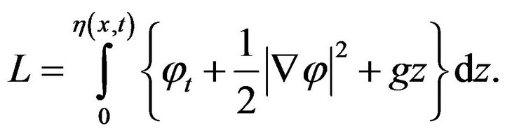(1)

The relevant ingredients, needed in order to describe this flow, are:

is the velocity potential, ρ is the fluid density, g is the acceleration by the Earth’s gravity, x is the horizontal coordinate, x-axis represents undisturbed surface with constant depth H, z is the vertical coordinate, is the elevation of the free surface.

Free surface is the surface of a fluid that is subject to constant perpendicular normal stress and zero parallel shear stress, such as the boundary between two homogenous fluids, for example liquid water and the air in the Earth’s atmosphere. Unlike liquids, gases cannot form a free surface on their own. A liquid in a gravitational field will form a free surface if unconfined from above. Under mechanical equilibrium this free surface must be perpendicular to the forces acting on the liquid; if not there would be a force along the surface, and the liquid would flow in that direction. Thus, on the surface of the Earth, all free surfaces of liquids are horizontal unless disturbed (except near solids dipping into them, where surface tension distorts the surface locally). In a free liquid at rest, that is, one subject to internal attractive forces only and not affected by outside forces such as a gravitational field, its free surface will assume the shape with the least surface area for its volume—a perfect sphere.

Now are allowed to vary subject to the restrictions 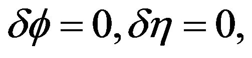on the boundary of D.

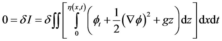
According to the standard procedure of the calculus of variations, Hamilton’s principle gives

Now

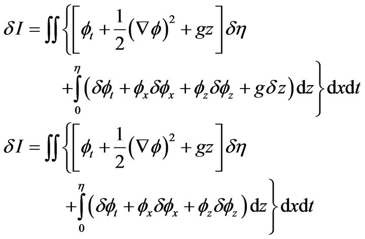
since.

Integrating the z-integral by parts, it turns out that

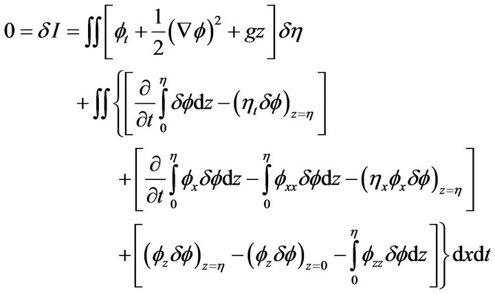
In view of the fact that the first z-integral in each of the square brackets vanishes on the boundary of D, we obtain

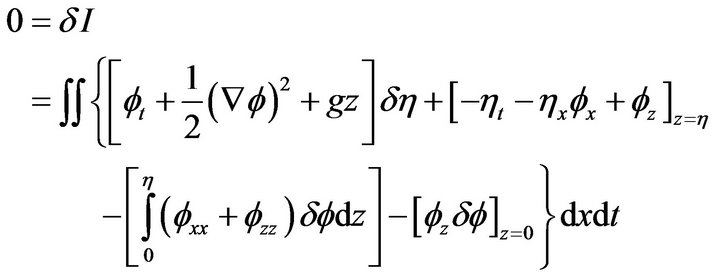
We first choose; since is arbitrary, we deduce

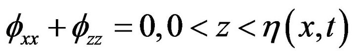
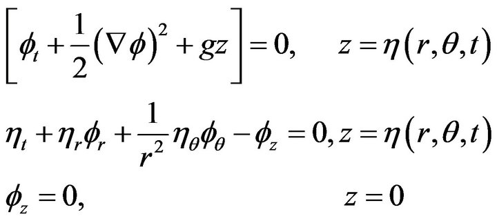
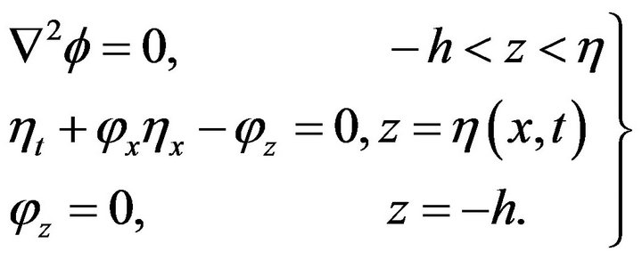
Then, since 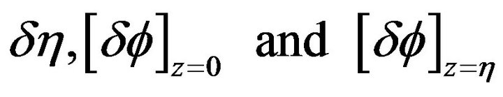can be given arbitrary independent values, we obtain

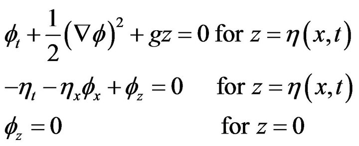
Evidently the Laplace equation, two free surface conditions, and the bottom boundary condition constitute the two-dimensional water wave equation. This system of equation has been used by Stoker [17], Debnath [18] for the investigation of the linearized initial value problem for the generation and propagation of water waves.

3. Water Wave Equation in Cylindrical Coordinates

We consider an inviscid irrotational flow of constant density subjected to a gravitational field g acting in the negative z-axis which is directed vertically downward. The fluid with a free surface is confined in a region. There exists a velocity potential such that the fluid velocity is given by 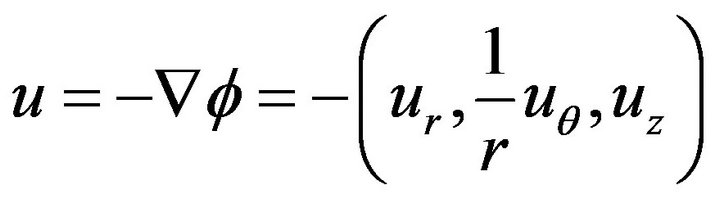the potential is lying between and. Then Hamilton’s principle with Lagrange function

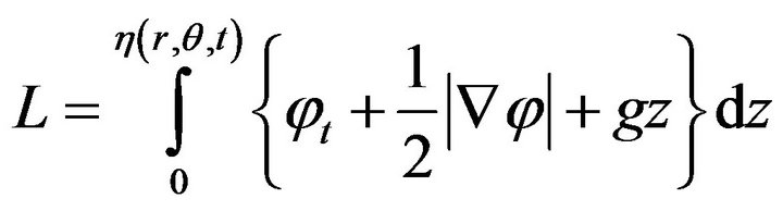(2)

and 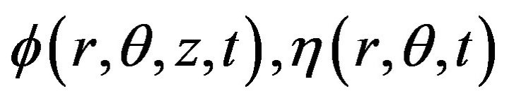are allowed to vary subject to the restrictions on the boundary δD of D.

According to the standard procedure of the Calculus of variations, Hamilton’s principle becomes

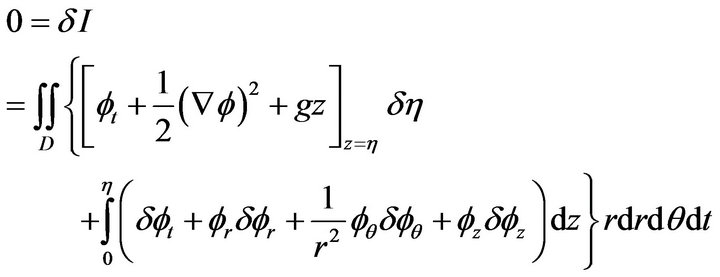
Integrating the z-integral by parts along with r and integrals, it turns out that

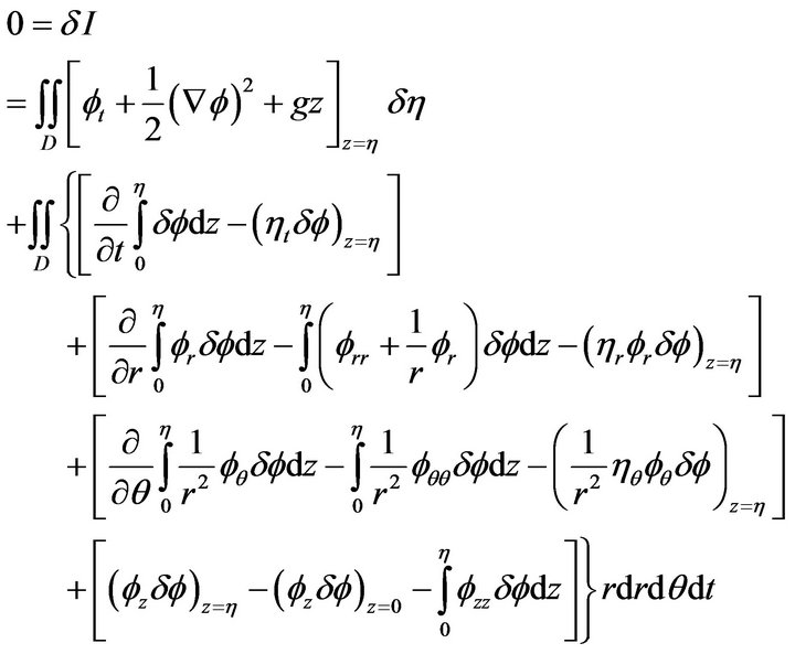
In view of the fact that the first z-integral in each of the square bracket vanishes on the boundary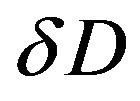, we obtain

We first choose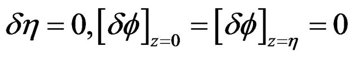; since is an arbitrary, we derive

Then since can be given arbitrary independent values, we deduce

Evidently, the Laplace equation, two flee-surface conditions and the bottom boundary condition constitute the non-axisymmetric water wave equations in cylindrical polar coordinates. This set of equations has also been used by several authors including Debnath [19], Mondal [20] and Mohanti [21] for the initial value investigation of linearized axisymmetric water wave problems.

4. Linear, Non-Rotating Shallow Waters

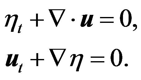
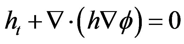
In non-dimensional form, the shallow-water equations take the form

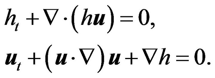
Here h represents the height of the free-surface, and the horizontal velocity field. The height h has been normalized by its mean value H, the velocity field by the characteristic speedConsidering and and are much smaller than one.

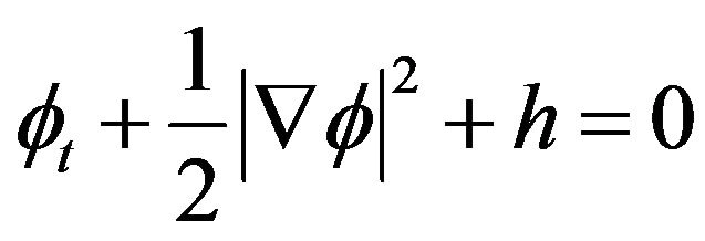
Hence we focus our attention here to irrotational flows. These are described by a scalar potential. For such flows,

(3)

(4)

where Lagrange function is

(5)

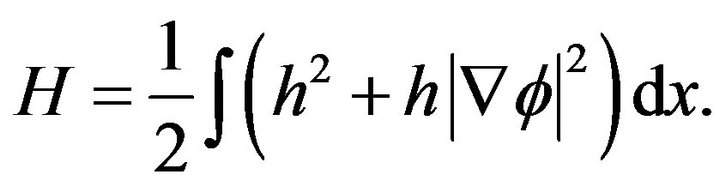
This system is Hamiltonian, with

(6)

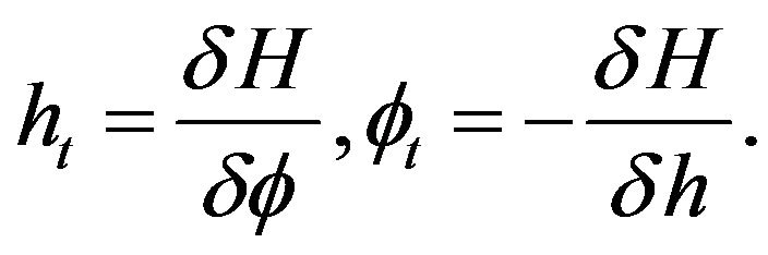
The Hamiltonian form of the equations is

(7)

5. Nonlinear, Non-Rotating Shallow Waters

For the fully nonlinear shallow-water equations, waves and vorticity no longer decouple. However, it is still true that a flow which starts irrotational stays so forever. Hence we may restrict ourselves to introduce again the scalar potential, and this will take the form

(8)

(9)

where Lagrange function is

(10)

This system is also Hamiltonian, with

(11)

and canonical equations

In this case, the Hamiltonian is the sum of the potential and kinetic energy.

6. Linear Water Wave Theory

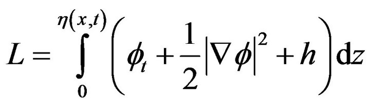
Here Hamilton’s Principle for irrotational water waves free of side conditions is used with Lagrange function

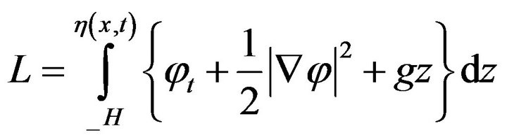(12)

Then, we have variation of within the flow region

(13)

The variation of gives the dynamical boundary condition on the free surface:

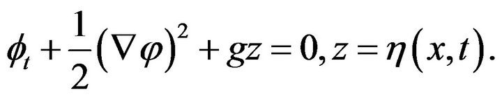(14)

7. Mathematical Formulation

Hongli et al. [16] derived these solutions to obtain water wave equation using variational principle.

(15)

where is a constant.

(16)

Here we consider,

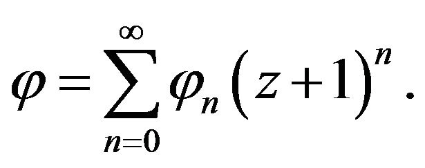(17)

From Laplace equation using Equation (17), we obtain

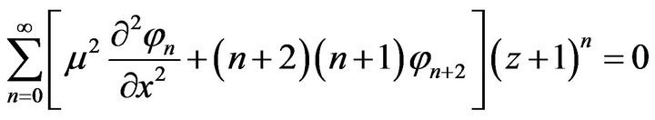(18)

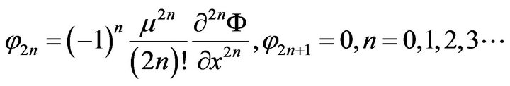
Since z be an arbitrary value within the flow region, so each coefficient in power of must be zero, thus

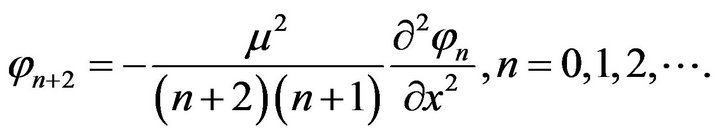(19)

On the other hand, using Equation (17) on the last free surface condition yields. Therefore, for all odds, , i.e.,

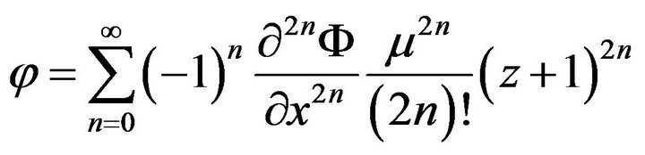
Supposing that, we have

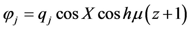
Now, the expression of velocity potential is obtained:

By linear approximation, we also consider

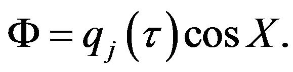(20)

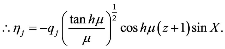
Therefore, the velocity potential can be found to be:

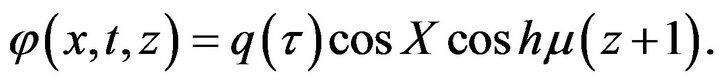
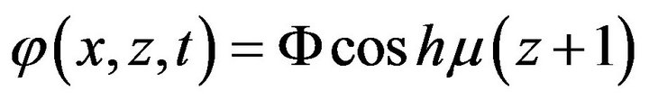using Equation (20)

Now

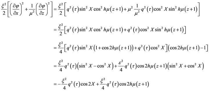
(21)

The case of, was considered by Benjamin [22] and Whitham [9], who obtained the Korteweg de Vries (KdV) equation. Here we also consider the case, and expand Lagrangian function up to order

(22)

Hou et al. [13] used the lowest-order of in their article.

Let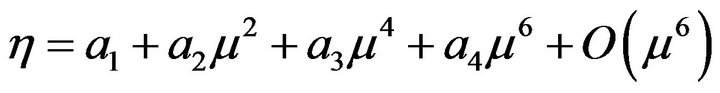

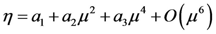
Expanding to th term, we have

Based on the dynamical boundary condition of the free surface, we have

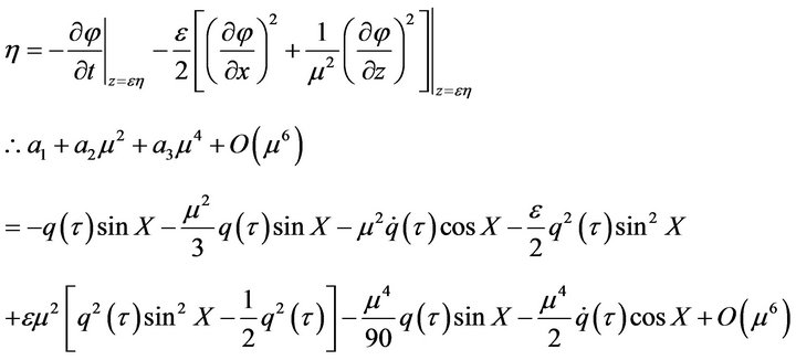(23)

From Equation (23), equating the coefficients of constant, and terms, we have

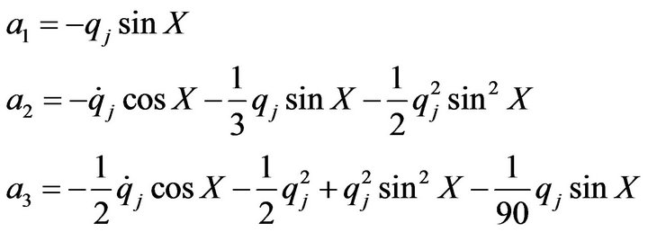(24)

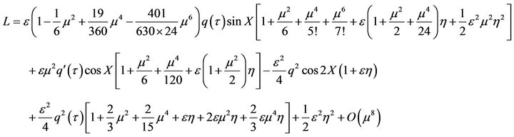
Substituting Equations (22) and (23) in Hamilton’s principle and neglecting the terms higher than order terms, we have the Lagrangian

Obviously, Lagrangian is a function of generalized coordinates and generalized velocity.

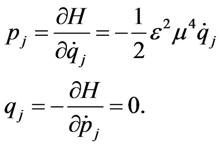
We also used the generalized momentum

Now Hamiltonian function

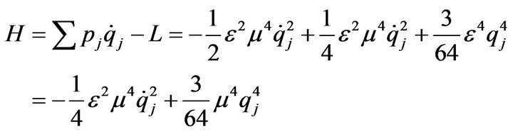
Hamilton’s canonical equation of motion

8. Conclusion

Firstly, we have generalized two dimensional water wave equation in Cartesian and in cylindrical polar coordinates. We have also discussed water wave equation with Lagrangian and Hamiltonian with canonical variables. Then the Lagrangian function within a certain flow region expanded up to. It is obvious that Lagrangian is a function of generalized coordinate and generalized velocity and Hamiltonian is the sum of kinetic energy and potential energy. Using generalized momentum Hamiltonian function is formulated and then Hamilton’s canonical equations of motion have been also developed.

REFERENCES

NOTES

^*Corresponding author.

REFERENCES

- G. B. Whitham, “A General Approach to Linear and Non-Linear Dispersive Waves Using a Lagrangian,” Journal of Fluid Mechanics, Vol. 22, No. 2, 1965, pp. 273- 283. doi:10.1017/S0022112065000745
- J. C. Luke, “A Variational Principle for a Fluid with a Free Surface,” Journal of Fluid Mechanics, Vol. 27, No. 2, 1967, pp. 395-397. doi:10.1017/S0022112067000412
- V. E. Zakharov, “Stability of Periodic Waves of Finite Amplitude on the Surface of a Deep Fluid,” Journal of Applied Mechanics and Technical Physics, Vol. 9, No. 2, 1968, pp. 190-194.
- A. C. Radder, “Hamiltonian Dynamics of Water Waves,” Advanced Series on Ocean Engineering, Vol. 4, 1999, pp. 21-59. doi:10.1142/9789812797551_0002
- R. Salmon, “Geophysical Fluid Dynamics,” Oxford University Press, Oxford, 1988.
- V. E. Zakharov and E. A. Kuznetsov, “Hamiltonian Formalism for Nonlinear Waves,” Physics Uspekhi, Vol. 40, No. 11, 1997, pp. 1087-1116. doi:10.1070/PU1997v040n11ABEH000304
- P. A. Madsen, H. R. Bingham and H. A. Schäffer, “Boussinesq-Type Formulations for Fully Non-Linear and Extremely Dispersive Water Waves: Derivation and Analysis,” Proceedings of the Royal Society of London, Vol. 459, No. 2033, 2003, pp. 1075-1104. doi:10.1098/rspa.2002.1067
- O. S. Madsen, S. Pahuja, H. Zhang and E. S. Chan, “A Diffusive Transport Mechanism for Fine Sediments,” Proceedings of the 28th International Conference on Coastal Engineering, Cardiff, 2003, pp. 741-753.
- G. B. Whitham, “Variational Methods and Applications to Water Waves,” Proceedings of the Royal Society A, Vol. 299, No. 1, 1967, pp. 6-25.
- J. W. Miles, “On Hamilton’s Principle for Surface Waves,” Journal of Fluid Mechanics, Vol. 83, No. 1, 1977, pp. 153-158. doi:10.1017/S0022112077001104
- D. M. Milder, “A Note Regarding ‘On Hamilton’s Principle for Surface Waves’,” Journal of Fluid Mechanics, Vol. 83, No. 1, 1977, pp. 159-161. doi:10.1017/S0022112077001116
- A. C. Radder, “An Explicit Hamiltonian Formulation of Surface Waves in Water of Finite Depth,” Journal of Fluid Mechanics, Vol. 237, 1992, pp. 435-455. doi:10.1017/S0022112092003483
- T. Y. Hou and P. Zhang, “Convergence of a Boundary Integral Method for 3-D Water Waves,” Discrete and Continuous Dynamical Systems, Series B, Vol. 2, No. 1, 2002, pp. 1-34. doi:10.3934/dcdsb.2002.2.1
- D. Ambrosi, “Hamiltonian Formulation for Surface Waves in a Layered Fluid,” Wave Motion, Vol. 31, No. 1, 2000, pp. 71-76. doi:10.1016/S0165-2125(99)00024-4
- Y. Lvov and E. G. Tabak, “A Hamiltonian Formulation for Long Internal Waves,” Physica D, Vol. 195, 2004, pp. 106-122. doi:10.1016/j.physd.2004.03.010
- Y. Hongli, S. Jinbao and Y. Liangui, “Water Wave Solutions Obtained by Variational Method,” Chinese Journal of Oceanology and Limnology, Vol. 24, No. 1, 2006, pp. 87-91. doi:10.1007/BF02842780
- J. J. Stoker, “Water Waves,” 1957.
- L. Debnath, “A Variational Principle for Nonlinear Water Waves,” Acta Mechanica, Vol. 72, No. 1-2, 1988, pp. 155- 160. doi:10.1007/BF01176549
- L. Debnath, “On Initial Development of Axisymmetrio Waves in Fluids of Finite Depth,” Proceedings of the National Institute of Sciences of India, Vol. 85, 1969, pp. 567-585.
- C. R. Mondal, “Uniform Asymptotic Analysis of Shallow-Water Waves Due to a Periodic Surface Pressure,” Quarterly of Applied Mathematics, 1986, pp. 133-140.
- N. C. Mahanti, “Small-Amplitude Internal Waves Due to an Oscillatory Pressure,” Quarterly of Applied Mathematics, Vol. 37, 1997, pp. 92-97.
- T. B. Benjamin, “Instability of Periodic Wavetrains in Nonlinear Dispersive Systems,” Proceedings of the Royal Society of London Series A, Vol. 299, No. 1456, 1967, pp. 59-76. doi:10.1098/rspa.1967.0123