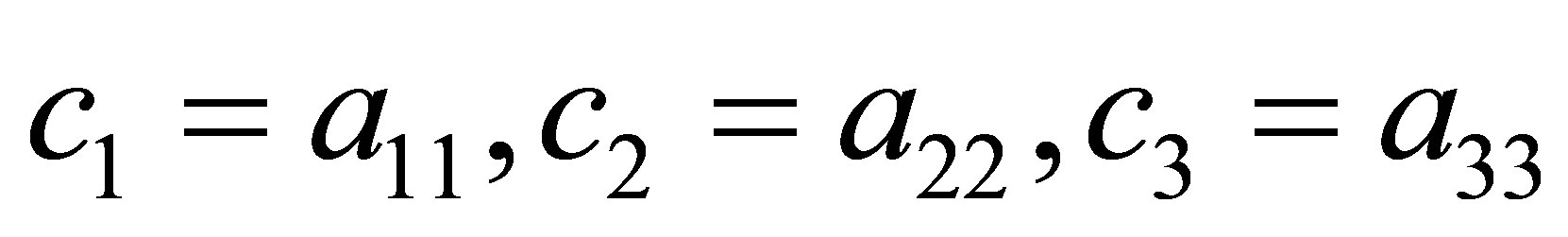
Advances in Linear Algebra & Matrix Theory
Vol.3 No.4(2013), Article ID:40924,10 pages DOI:10.4236/alamt.2013.34012
The Solution of the Eigenvector Problem in Synchrotron Radiation Based Anomalous Small-Angle X-Ray Scattering
Institute of Soft Matter and Functional Materials, Helmholtz-Zentrum-Berlin, Berlin, Germany
Email: guenter.goerigk@helmholtz-berlin.de
Copyright © 2013 Guenter Johannes Goerigk. This is an open access article distributed under the Creative Commons Attribution License, which permits unrestricted use, distribution, and reproduction in any medium, provided the original work is properly cited.
Received October 22, 2013; revised November 22, 2013; accepted November 29, 2013
Keywords: Matrix Inversion; Eigenvalues; Eigenvectors; Pair Correlation Functions; Basic Scattering Functions
ABSTRACT
In the last three decades Synchrotron radiation became an indispensable experimental tool for chemical and structural analysis of nano-scaled properties in solid state physics, chemistry, materials science and life science thereby rendering the explanation of the macroscopic behavior of the materials and systems under investigation. Especially the techniques known as Anomalous Small-Angle X-ray Scattering provide deep insight into the materials structural architecture according to the different chemical components on lengths scales starting just above the atomic scale (≈1 nm) up to several 100 nm. The techniques sensitivity to the different chemical components makes use of the energy dependence of the atomic scattering factors, which are different for all chemical elements, thereby disentangling the nanostructure of the different chemical components by the signature of the elemental X-ray absorption edges i.e. by employing synchrotron radiation. The paper wants to focus on the application of an algorithm from linear algebra in the field of synchrotron radiation. It provides a closer look to the algebraic prerequisites, which govern the system of linear equations established by these experimental techniques and its solution by solving the eigenvector problem. The pair correlation functions of the so-called basic scattering functions are expressed as a linear combination of eigenvectors.
1. Introduction
Small-Angle X-ray Scattering (SAXS) experiments average over a large sample volume and give structural and quantitative information of high statistical significance on a mesoscopic length scale between 1 and hundreds of nanometers, which can be correlated to the macroscopic physical and chemical properties of the analysed condensed matter systems in solid state physics, chemistry, life science and materials science. Detailed descriptions of the experimental and theoretical aspects of Small-Angle Scattering can be found in [1-3]. By use of synchrotron radiation at suitable storage rings the socalled Anomalous Small-Angle X-ray Scattering (ASAXS) can be employed, which is an excellent tool for the chemical selective structural analysis of multi-component systems.
This publication outlines in detail the basic mathematical aspects related to the scientific results of a series of former publications [4-16] obtained from quantitative ASAXS measurements applied to very different physicochemical systems. The quantitative analysis of the nano-scaled phases is correlated with the structural parameters, via the pair correlation functions and the socalled basic scattering functions, which provide (by Fourier transform) the nano-scaled architecture with very high statistical significance because scattering experiments average over up to 1010 structural entities. The related scientific problems cannot be addressed by a classical Small-Angle X-ray Scattering (SAXS) experiment, because the specific scattering contributions of the different chemical components need to be separated. As outlined in a former publication [12] an outstanding experimental accuracy is needed in order to separate the so-called pure-resonant (element specific) scattering contribution. Additionally a suitable mathematical algorithm is employed (the Gauss elimination algorithm), which turned out to provide the best results when inverting the vector equation introduced by ASAXS measurements. The paper wants to shed some light on the algebraic basics, which govern the analysis of numerous ASAXS publications within the last decade.
2. The Eigenvector Problem Established by Anomalous Small-Angle X-Ray Scattering
2.1. Anomalous Small-Angle X-Ray Scattering
The remarkable possibilities of the ASAXS technique are based on the energy dependence of the atomic scattering factors giving selective access to the specific SAXS contributions of nano-scaled phases, which are built up by different chemical constituents in composites like for instance alloys, chemical solutions or porous multicomponent systems. In general the atomic scattering factors are energy dependent complex quantities:
 (1)
(1)
where Z represents the atomic number. When performing ASAXS measurements on multi-component systems in the vicinity of the absorption edge of one of the sample constituents the scattering amplitude is:
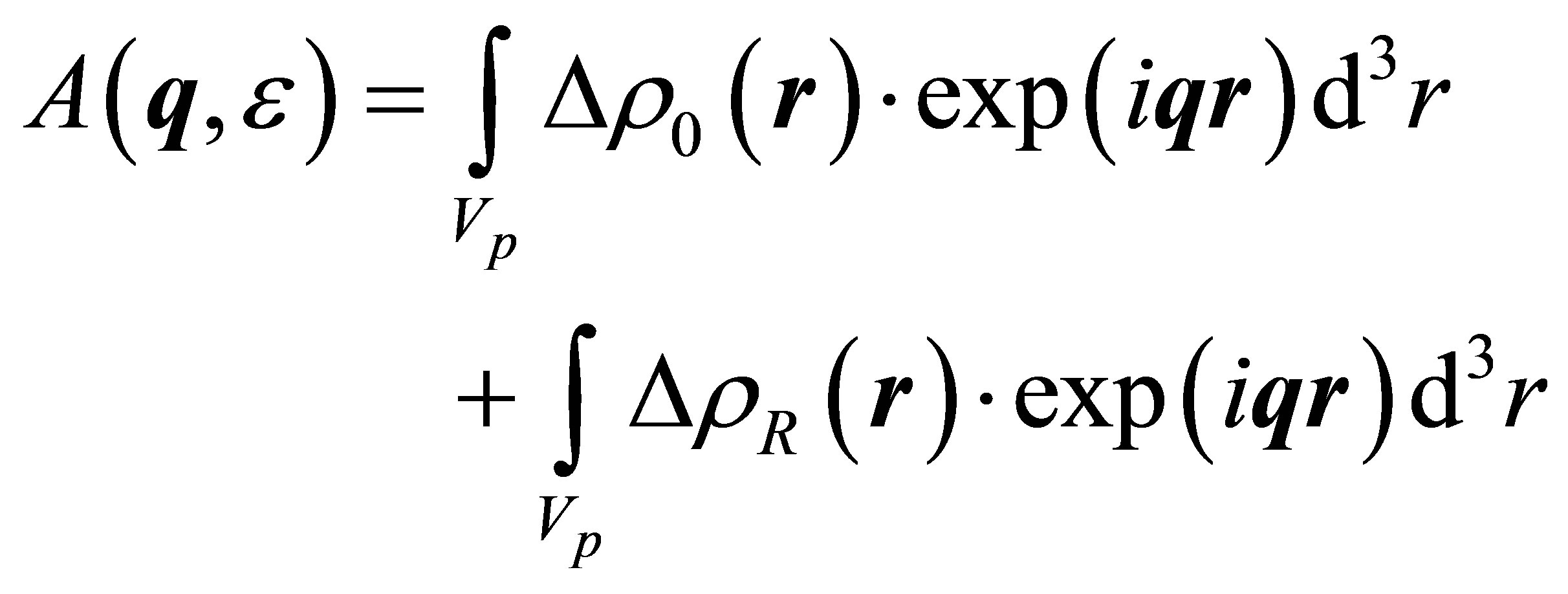 , (2)
, (2)
where q is the magnitude of the scattering vector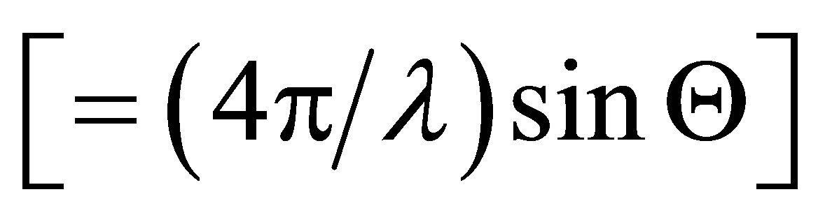 ,
, 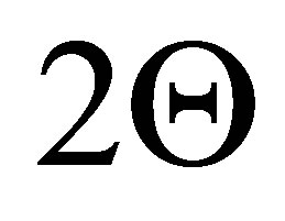 is the scattering angle, λ the X-ray wavelength and Vp is the irradiated sample volume.
 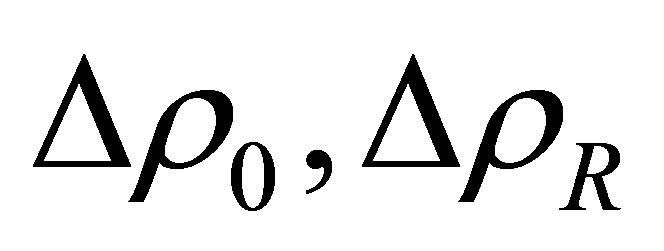 are the differences of electron densities of the non-resonant and the resonant scattering atoms,
 (3)
(3)
calculated from the electron density,  , and the atomic (molecular) volumes
  and
and , respectively, where
  is the electron density of the entire sample. The volume
  represents the atomic (molecular) volume of the non-resonant scattering atoms or building groups.
  corresponds to the atomic volumes of the resonant scattering atoms. The functions
  are the number densities of the non-resonant and the resonant scattering units, respectively and represent their spatial distribution in the sample. The atomic scattering factor,
  , is nearly energy independent, while the atomic scattering factor,
  , shows strong variation with the energy in the vicinity of the absorption edge of the resonant scattering atoms due to the so-called anomalous dispersion corrections
 . Calculating the scattering intensity
 by means of Equations (2) and (3) and averaging over all orientations yields the sum of three scattering contributions,
  , with the convolution integrals [17,18]:
 (4)
(4)
Equation (4) gives the so-called non-resonant scattering,  , the cross-term or mixed-resonant scattering,
  , originating from the superposition of the scattering amplitudes of the non-resonant and the resonant scattering atoms and finally,
  , which contains only the scattering contributions of the resonant scattering atom species. These basic scattering functions are based on the pair correlation functions
 ,
,  ,
,  and in the literature are sometimes referred to as Stuhrmann functions.
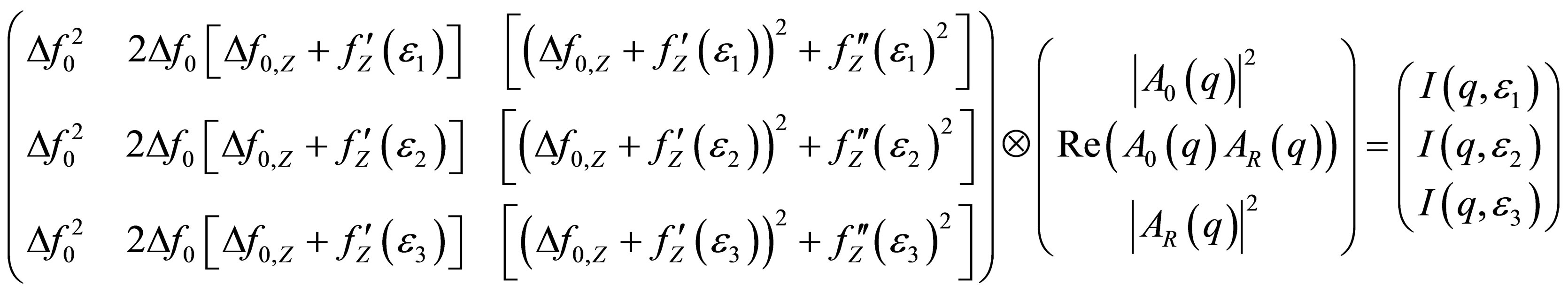
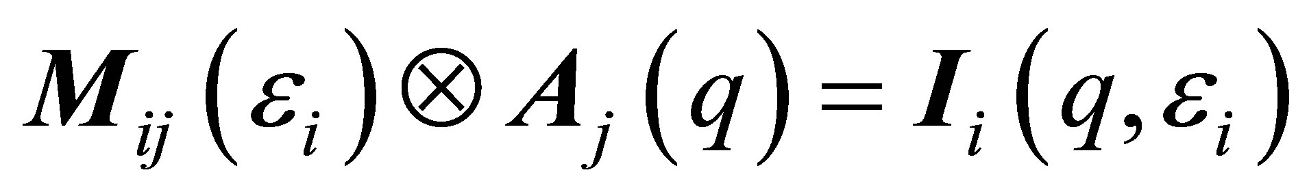
The measurement of scattering curves at three energies in the vicinity of the absorption edge of the atoms with atomic number Z constitutes the following vector equation:
 , (5)
, (5)
where the summation is running over the index j of the matrix and vector components.
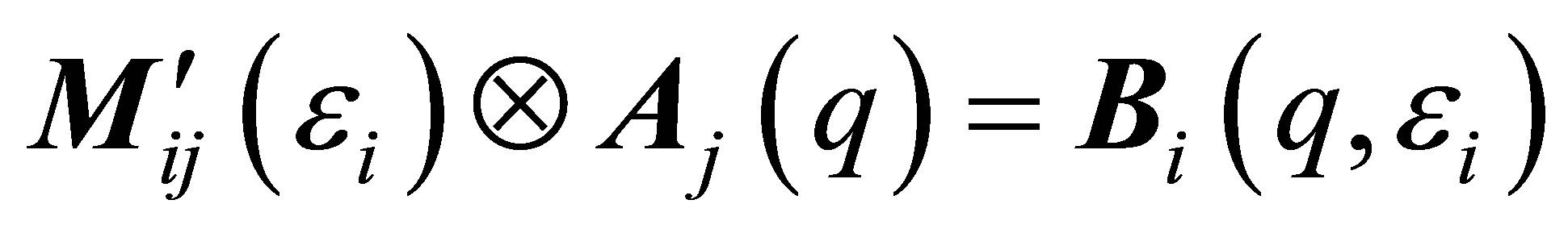
 (5a)
(5a)
with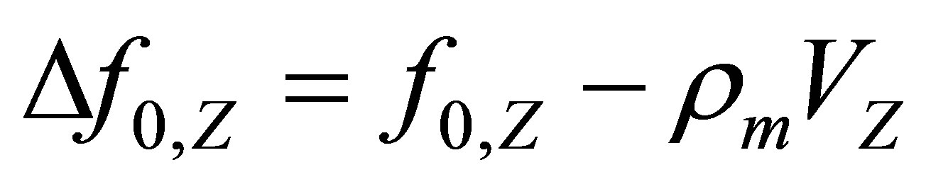 . The summation is running over the index j i.e. summing over the vector components Aj and the columns of the matrix Mij in the row with index i. The transformation of the vector Equation (5) by elementary operations changes the matrix M into the triangular matrix M':

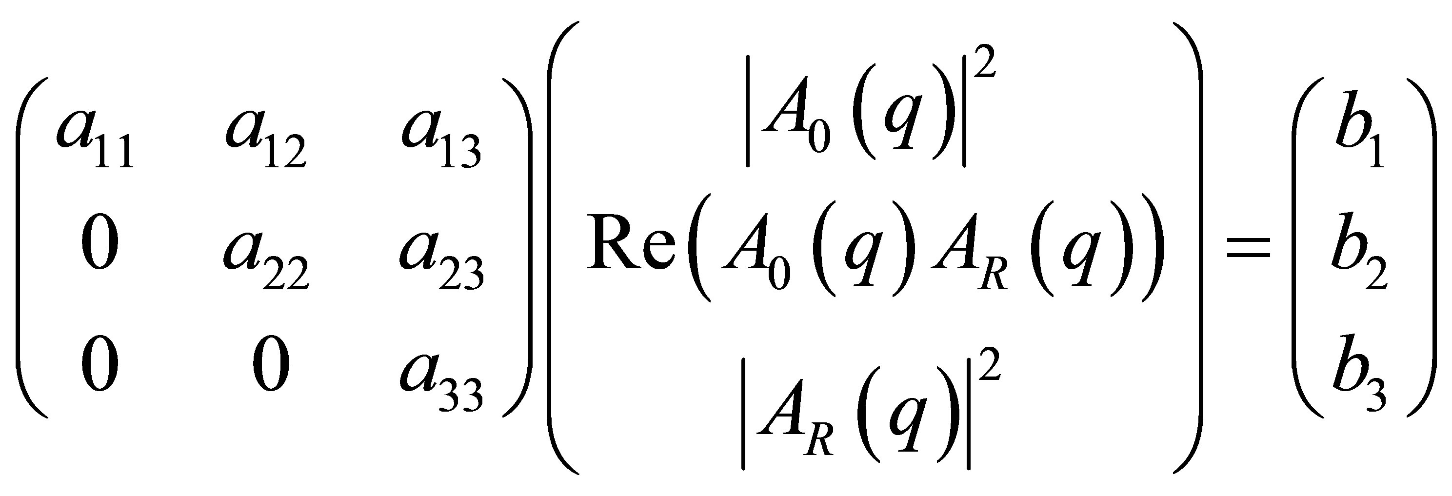 (6)
(6)
where the meaning of 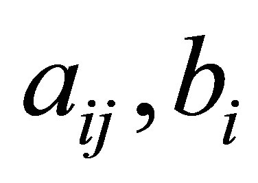 is [11]:
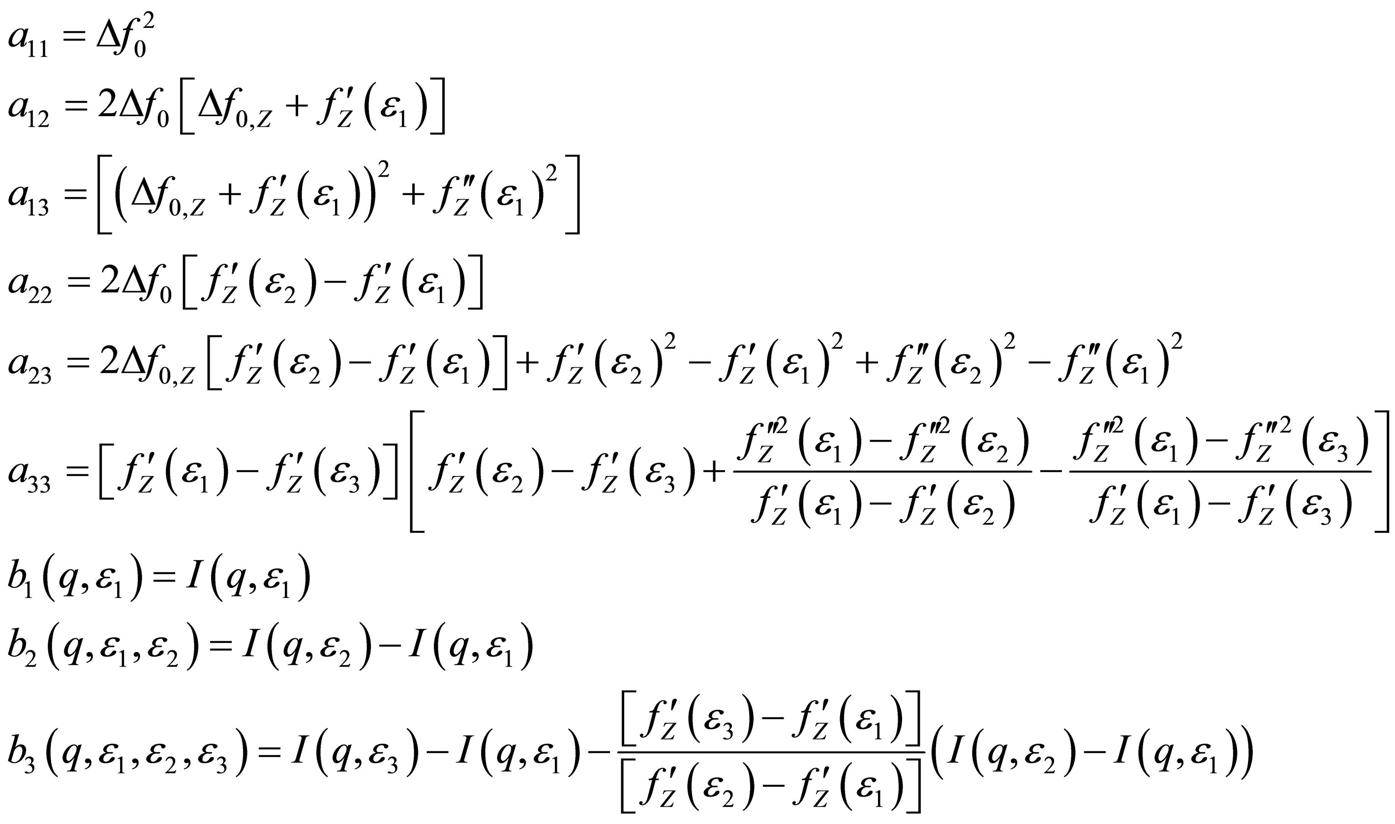 (7)
(7)
The vector Equation (6) with the triangular matrix represents the Gauss algorithm (elimination procedure) for the solution of a system of linear equations. Thus the elimination procedure is equivalent to the elementary operations performed to the matrix of a vector equation.
2.2. The Eigenvector Problem in Anomalous Small-Angle X-Ray Scattering
Up to this point the Equations (1)-(7) have been taken from [11,14] and represent nothing new. In what is to follow the underlying basics of linear algebra and the high degree of significance obtained by a suitable matrix inversion applied to experimental data (here scattering curves) will be outlined. In detail we demonstrate the calculation of the eigenvalues of the vector Equation (6) from the characteristic polynomial thereby providing the eigenvectors. Furthermore the representation of the special solution as a linear combination of the eigenvectors is demonstrated. In the next step analytical expressions for the pair correlation functions have been deduced from the eigenvector representation. Finally in the last step the basic scattering functions (Stuhrmann functions) are provided.
We start with the vector Equation (6):  . The characteristic polynomial for the determination of the eigenvalues writes:
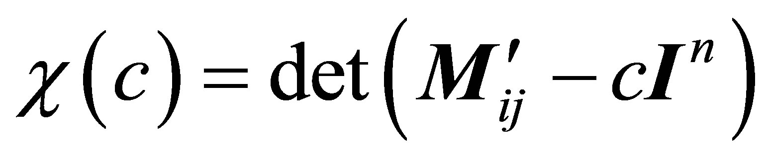 (8)
(8)
In represents the identity matrix:
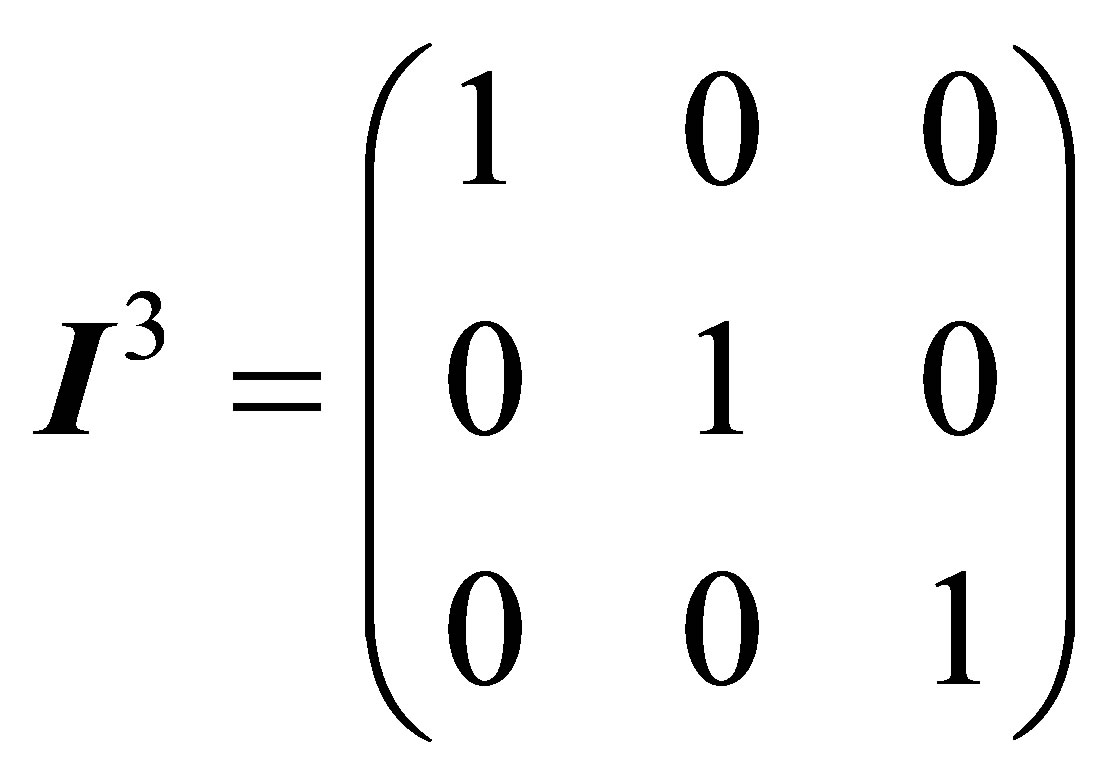 (9)
(9)
We will restrict the problem to n = 3, which is the minimum number of energies to be measured in order to solve the system of linear equations with three unknown quantities. From Equations (8) and (9) the polynomial is deduced:
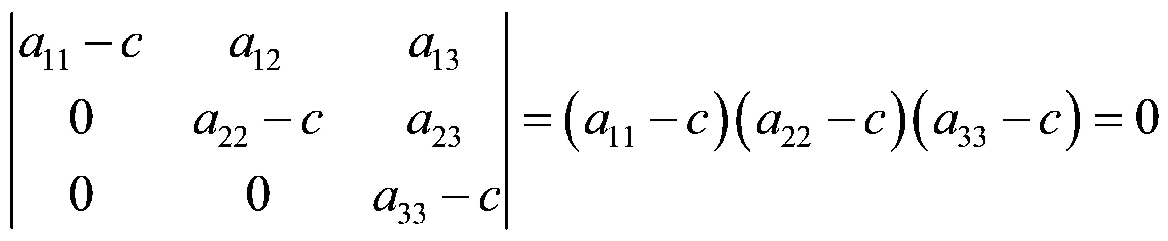 (10)
(10)
giving the three eigenvalues:
 (11)
(11)
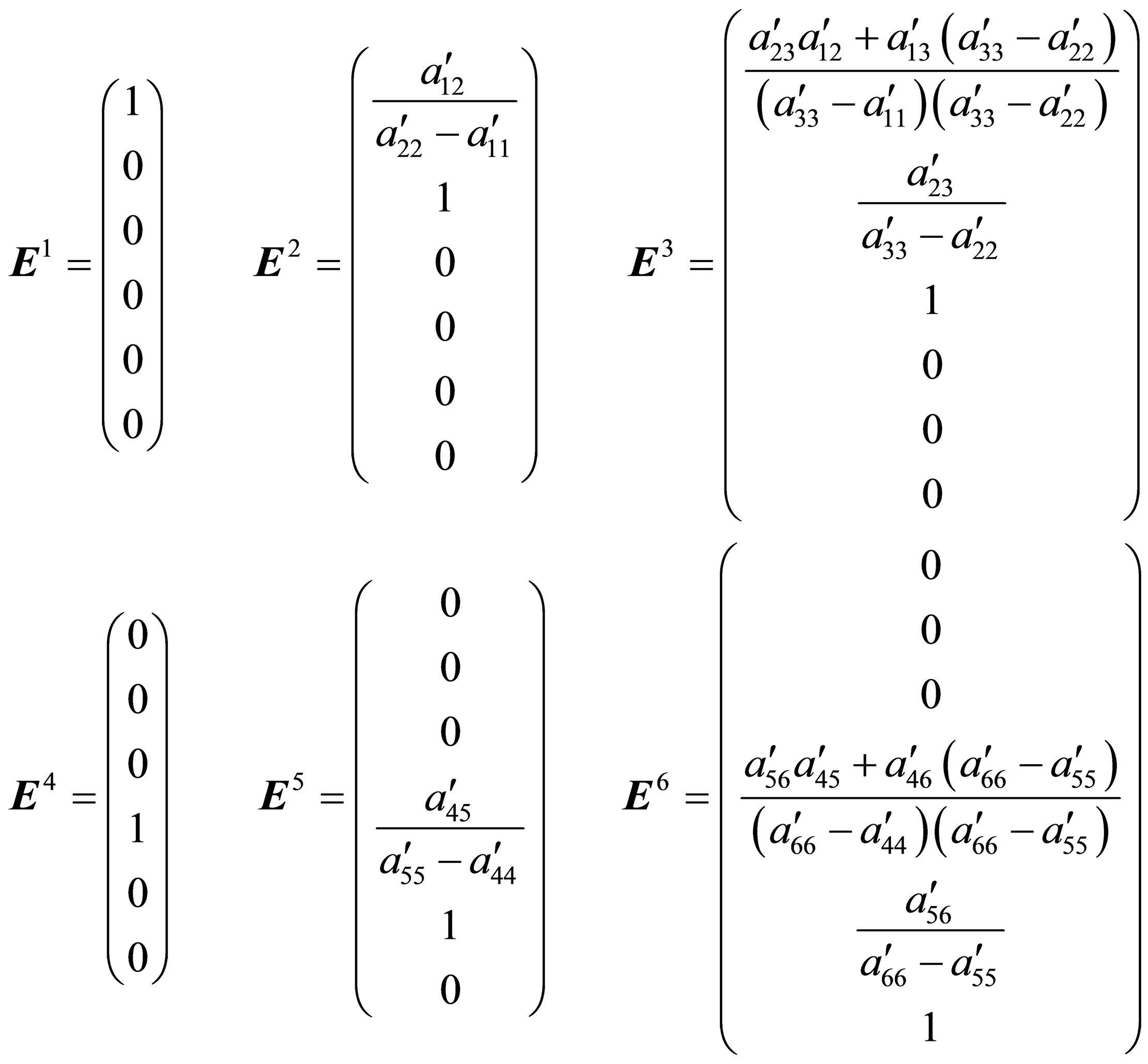
From the eigenvalues the eigenvectors, Ei, can be constructed via Equation (12):
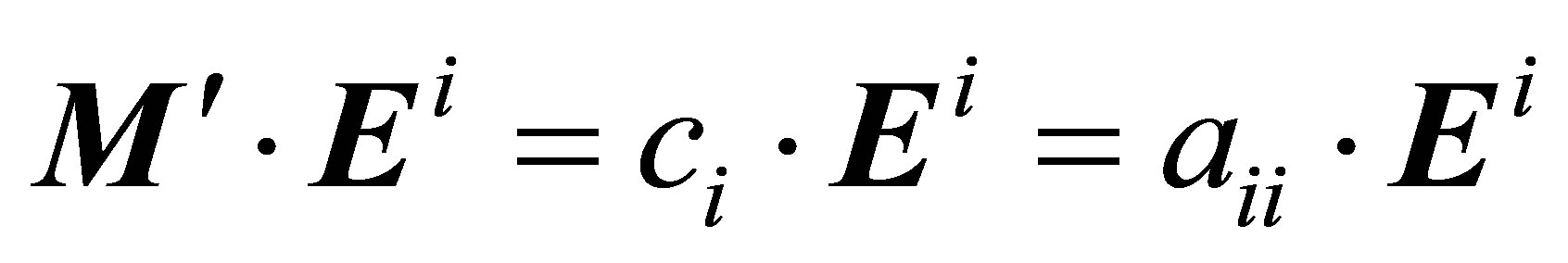 , (12)
giving:
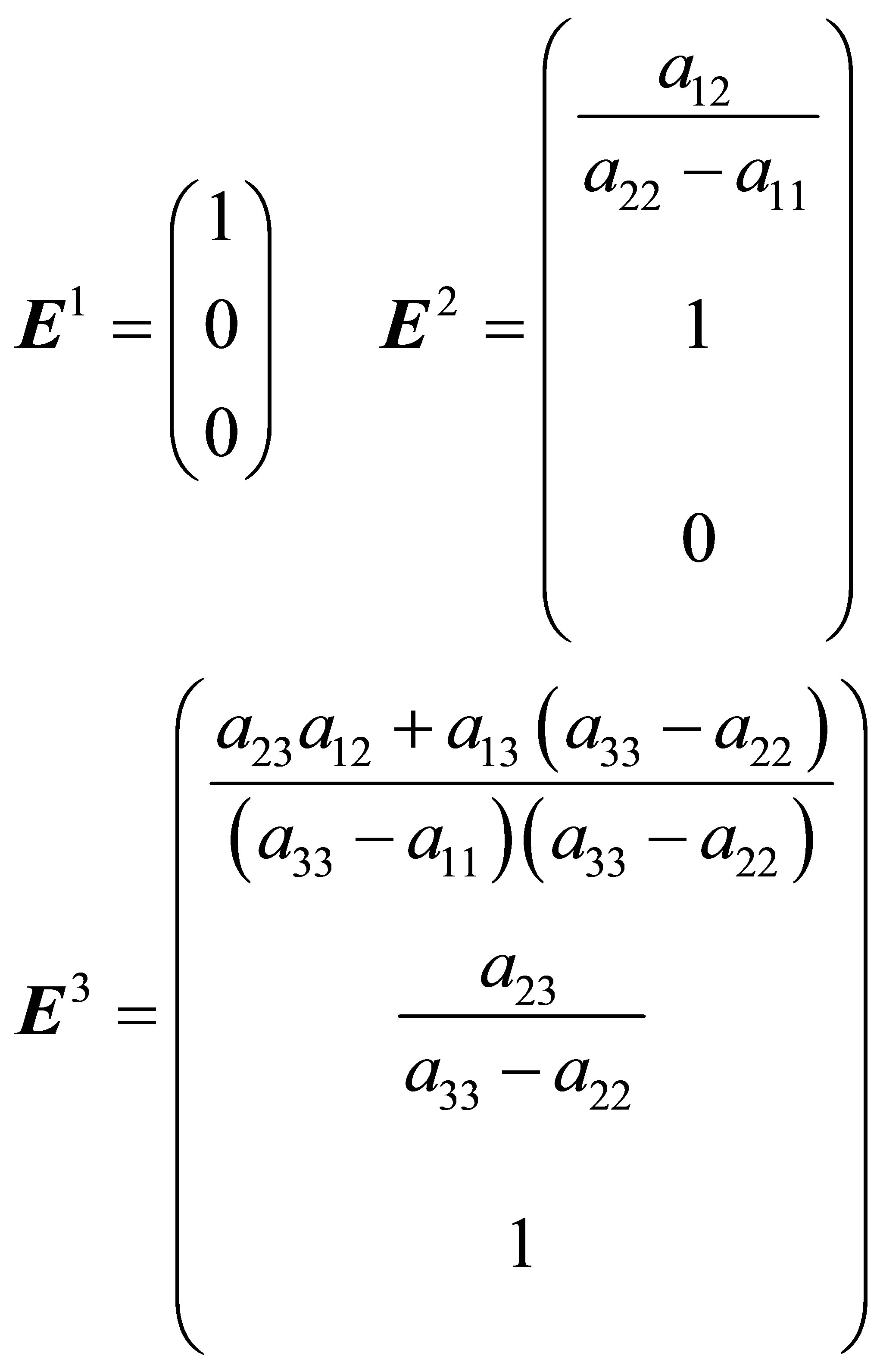 (13)
(13)
Because these eigenvectors are linear independent they define a system of basic vectors in the solution space and the vectors A and B can be expressed via a linear combination of the eigenvectors Ei:
 (14)
(14)
Thus the vector composed from the pair correlation functions can be represented by a linear combination of the eigenvectors Ei with the linear coefficients xi. From the vector Equation (14) the linear coefficients xi can be calculated:
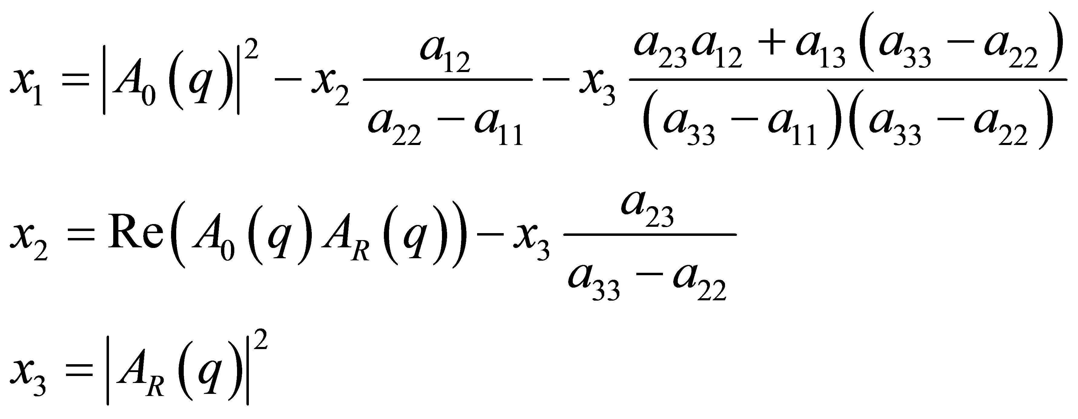 (15)
(15)
In the next step Equation (14) is inserted into Equation (6):
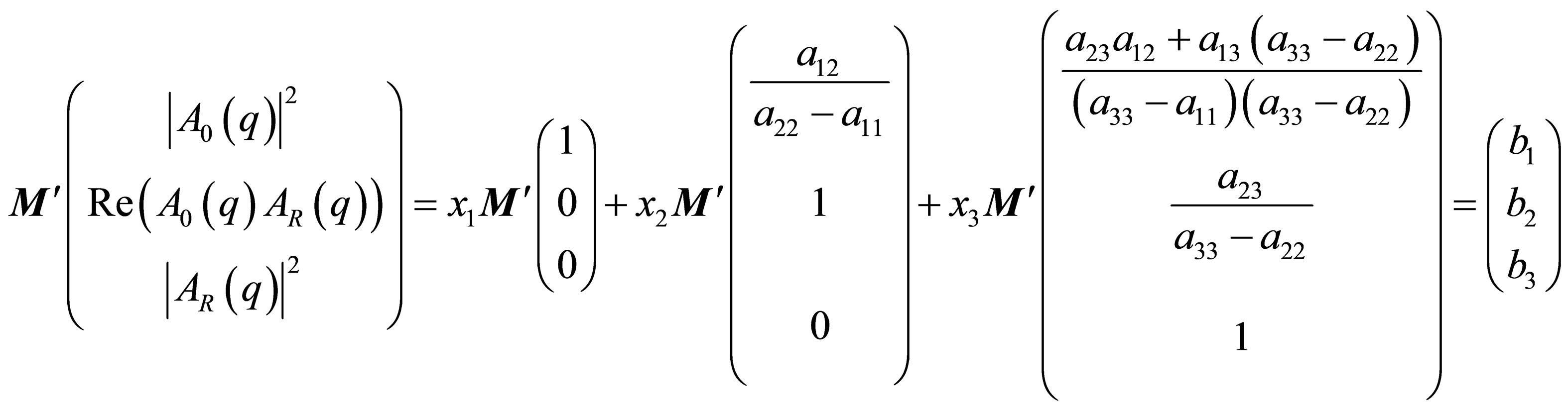 (16a)
(16a)
or, because the Ei are eigenvectors of M':
 (16b)
(16b)
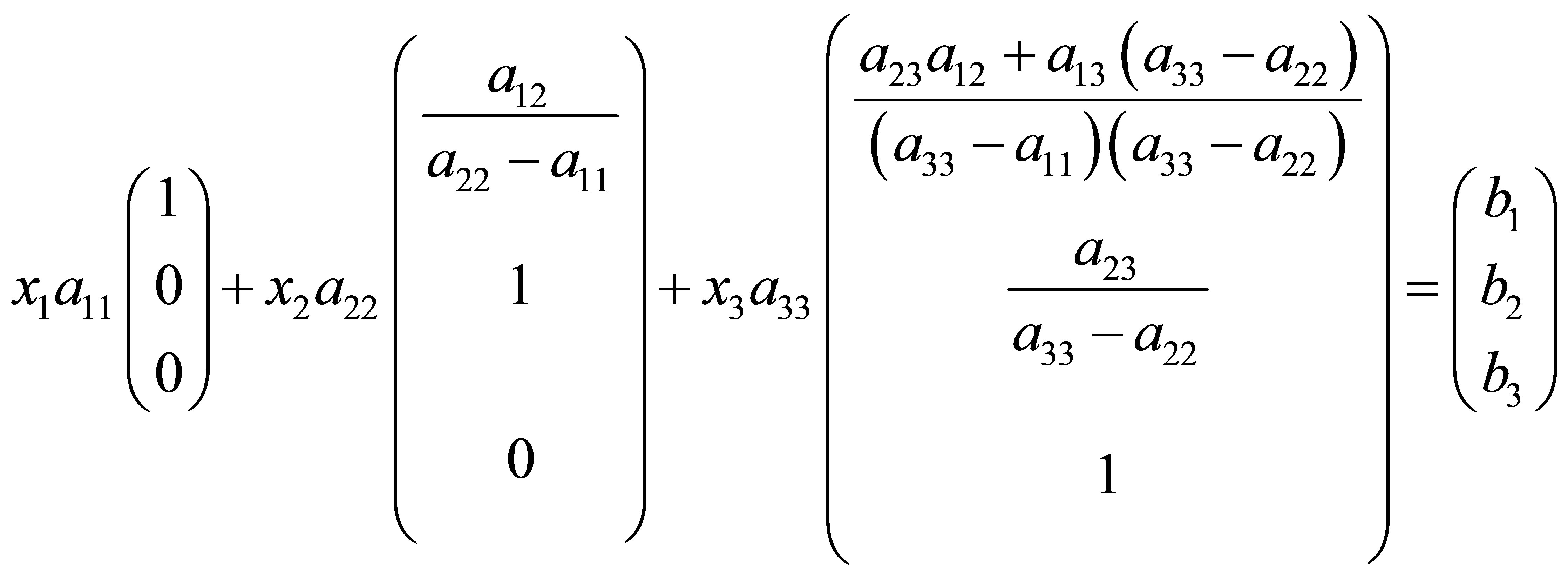
From the vector Equation (16b) the three pair correlation functions can be calculated by inserting the xi from Equation (15) into Equation (16b):
 (17)
(17)
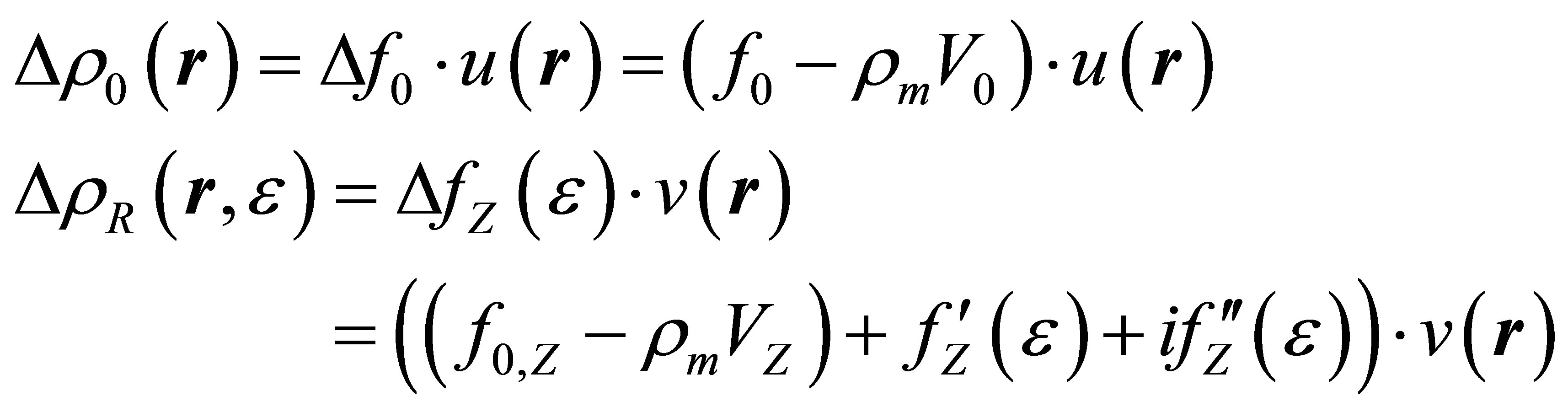
Figure 1 summarizes the results from Equations (1) to (17). The three pair correlation functions ,
,  ,
,  are plotted along the three rectangular axis of the 3-dimensional coordinate system. The eigenvectors E1, E2(ε), E3(ε) build up an obliqueangled coordinate system where two of them depend on the photon energy. The blue and the red line show the eigenvectors E2(ε) and E3(ε) following curvatures depending on the energy via their vector components. Thus the pair correlation functions of Equation (14) depicted by the black vector are represented by the parallelepiped
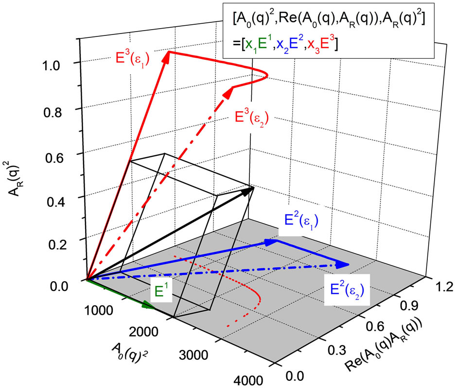
Figure 1. The pair correlation functions (black vector) in eigenvector representation. The eigenvectors E1 (green) E2 (blue) and E3 (red) build up the oblique-angled coordinate system (see text). The parallelepiped depicts the black vector in eigenvector representation at energy ε1. For energy ε2 the dashed blue and red vectors together with the energy independent vector E1 (green) are the eigenvectors. The underlying data of the red and the blue curves have been taken as example from Cromer Liberman calculations [21,22] of the LIII-absorption edge of Thallium. Note the different length scales of the 3 axis in the rectangular basic system. In order to depict the energy dependence of the eigenvectors with a better resolution the x-component of E2 and the y-component of E3 have been stretched by a factor 100 and 10 respectively. For the same reason the x-component of E3 was compressed by a factor of 10 and E1 is stretched by a factor 1500. Δf0 = −3.5. The dashed red line represents the projection of E3(ε) onto the grey xy-plane.
which shows the vector of pair correlation functions in eigenvector representation with the coordinates xi/li in the oblique angled basic system. The li are the lengths of the basic vectors Ei.
From Equation (17) the so-called basic scattering functions (Stuhrmann functions) can be deduced (see Equation (4)):
 (18)
(18)
or in explicit form:
 (19)
(19)
Equation (19) provides the analytical form for the calculation of the basic scattering functions from scattering curves measured at in minimum three energies. The mathematical theory behind this formula is the solution of the eigenvalue problem in six steps:
1) Calculation of the triangular matrix by elementary operations upon the vector equation established by an ASAXS measurement at in minimum three different energies.
2) Calculation of the eigenvalues from the characteristic polynomial of the new vector equation obtained from the elementary operations.
3) Calculation of the eigenvectors.
4) Representation of both, the special solution vector Ai and the vector Bi by linear combination of the eigenvectors.
5) Calculation of the pair correlation functions,  ,
,  ,
,  from these representations.
6) Calculation of the basic scattering functions (Stuhrmann functions) from the basic pair correlation functions.
With the definition of S0R in Equation (4) the three basic scattering functions fulfill the Cauchy-Schwarz inequality because the integrals in S0, S0R and SR of Equations (4) and (20) define a positive definite metric in the vector space of functions [5,14]:
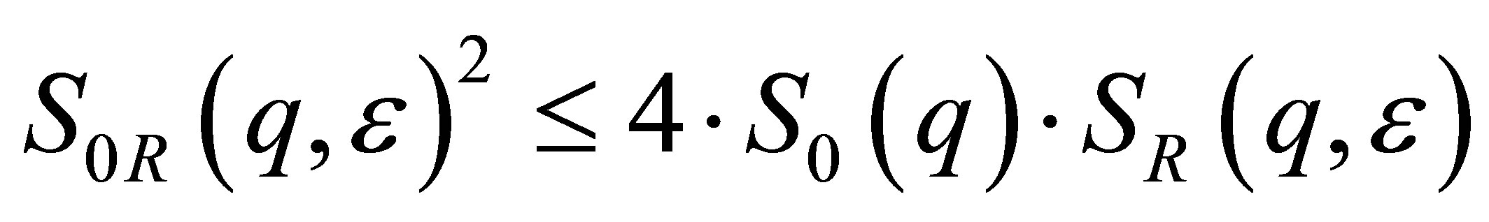 (20)
(20)
This criterion is essential but not sufficient for the reliability of the basic scattering functions obtained from the matrix inversion. If it is not fulfilled, the basic scattering functions are meaningless. The significance of the special solution obtained by matrix inversion can be numerically quantified by the Turing number [19]:
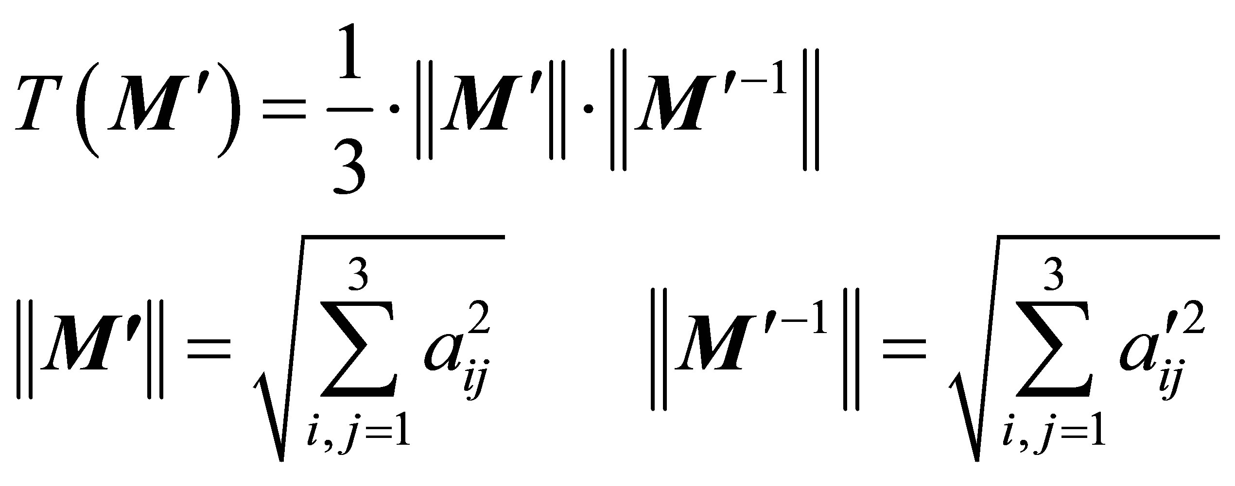 , (21)
where  is the inverse matrix. A detailed description of the impact of the Turing number for ASAXS measurements is given in [14,20].
2.3. The Eigenvector Problem in Anomalous Small-Angle X-Ray Scattering with More than Three Energies at One X-Ray Absorption Edge
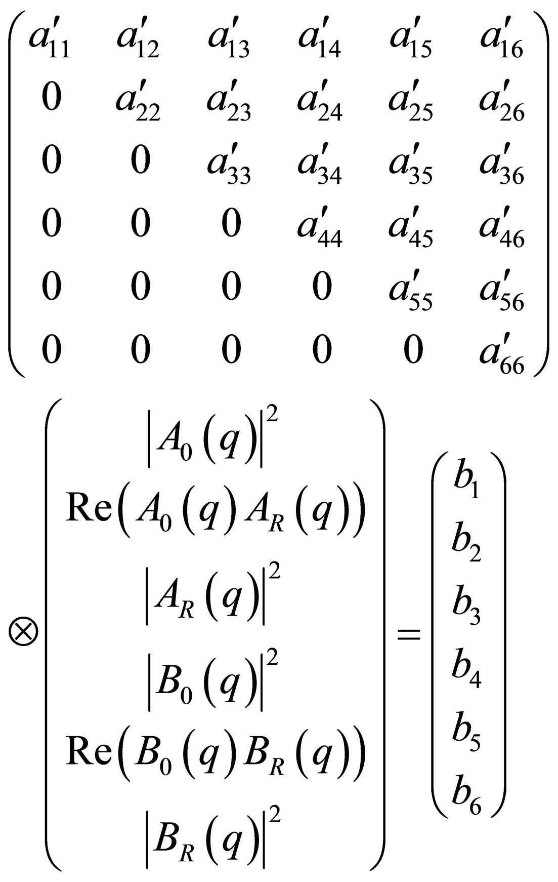
In the following we will discuss the system of linear equations with more than three (4…n) energies:
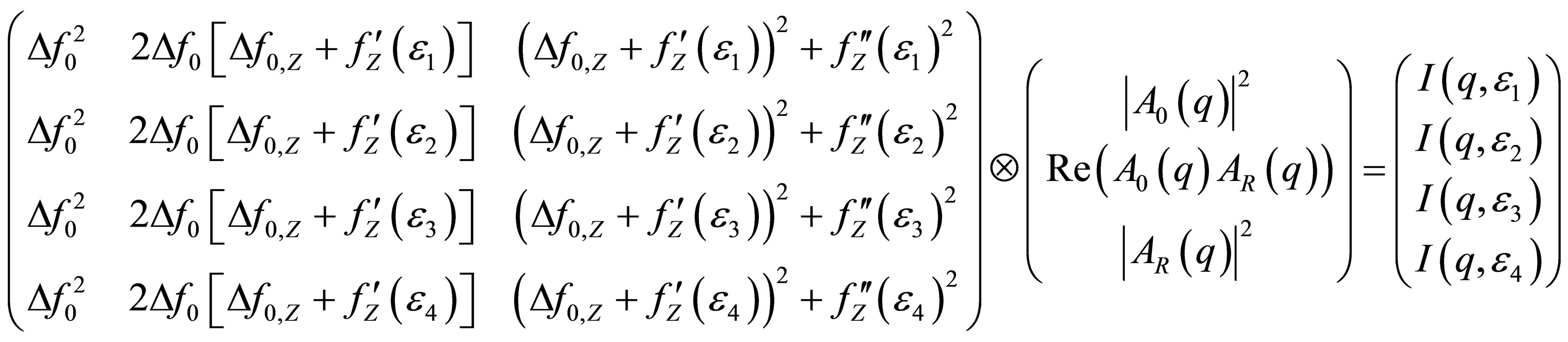 (22)
(22)
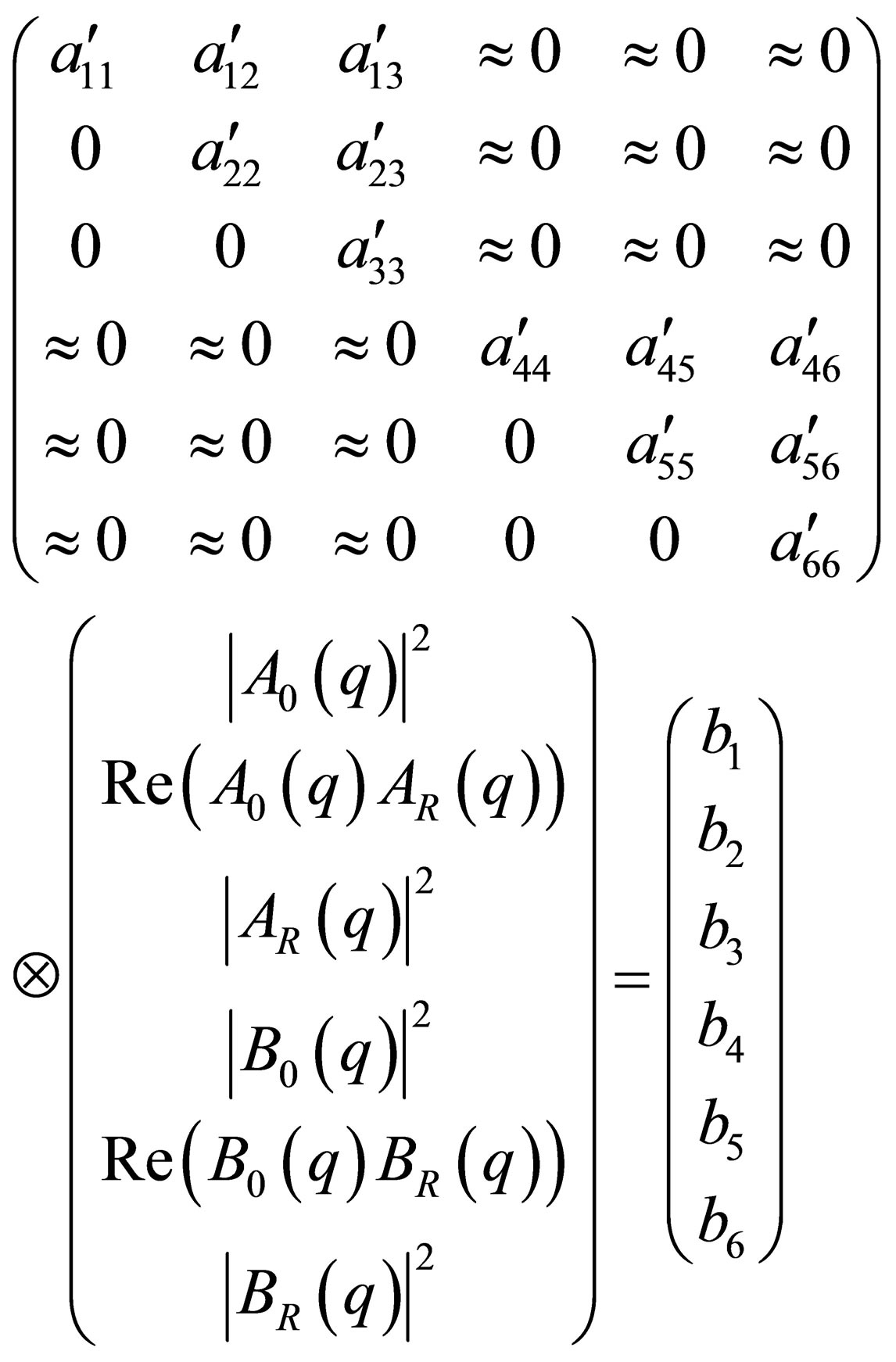
Equation (22) represents an ASAXS sequence with scattering curves I(q,εi) measured at four different energies εi. Once again the summation is running over the index j = 1, 2, 3 i.e. summing over the vector components Aj and the columns with index j of the rectangular i × j-matrix Mij in the row with index i. But now the resulting vector has four components on the right side. Equation (22) represents a linear map from a 3-dimensional space into a 4-dimensional space. The possible solutions are located in the 3-dimensional subspace, which is embedded in the 4- dimensional space. Because the rank of the matrix is three in minimum two of the four linear equations must be linear dependent. The transformation of the vector Equation (22) by elementary operations changes the matrix M into the triangular matrix M' of the form:
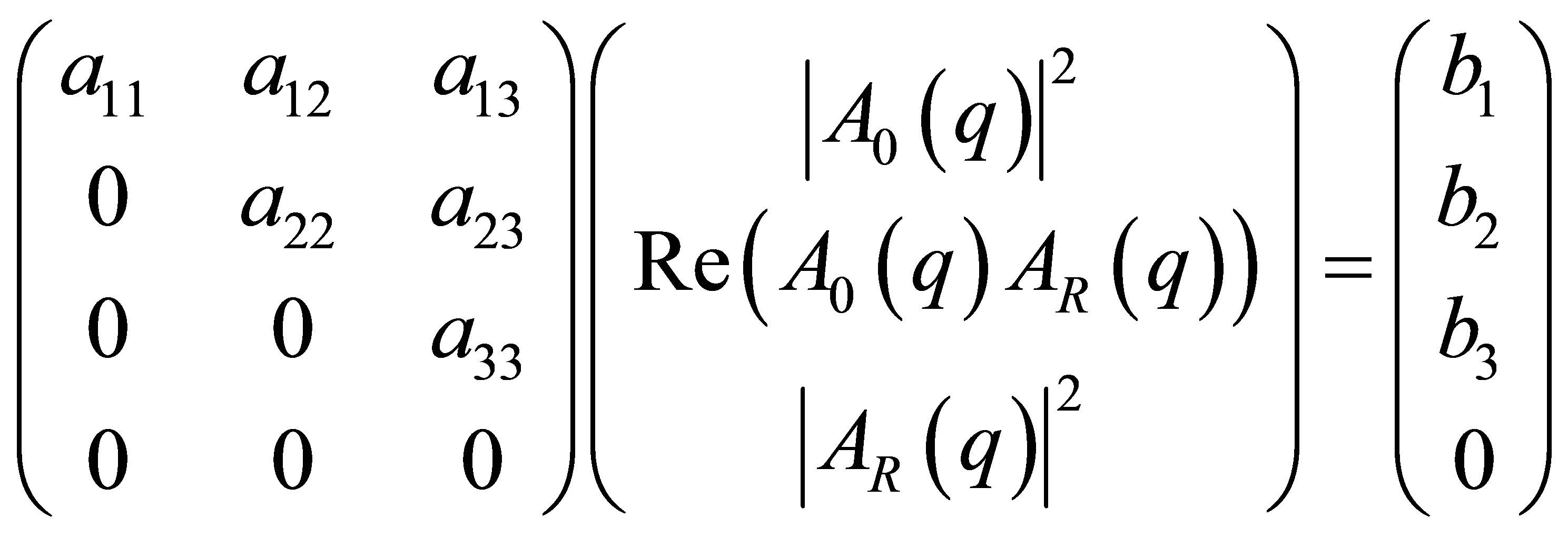 (23)
(23)
As a consequence the fourth component of the vector on the right side must be zero, b4 = 0. Of course when performing measurements the latter is not exactly fulfilled due to the error bars of the measurements. Thus the value of the fourth row is not exactly zero but nearly zero!
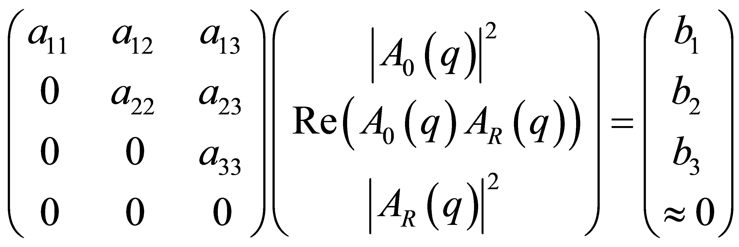 (24)
(24)
Because b4 is not exactly zero, the vector is located in the 4-dimensional space but outside the embedded 3- dimensional space of solution vectors. Thus no exact solution for the system of linear equations exists. Only an approximate solution exists. It is the vector in the 3-dimensional hyper plane with the shortest distance to B in the 4-dimensional space or in other words: the foot of the perpendicular constructed between B and the hyper plane (Figure 2). The meaning of Equation (24) is: no improvement can be obtained from additional measurements of scattering curves at more than three energies, because the rank of the matrix is three or in other words in case of more than three equations in the 3-dimensional vector space in minimum two of them are linear dependent. The same argumentation holds for n energies. The significance of the solution vector obtained by the matrix inversion of the system of linear equations can be calculated by the Turing number, which was outlined in a recent publication [14]. Note that the Turing number increases with the number n of equations (energies) by  i.e., ASAXS measurements at many (n > 3) energies cannot improve
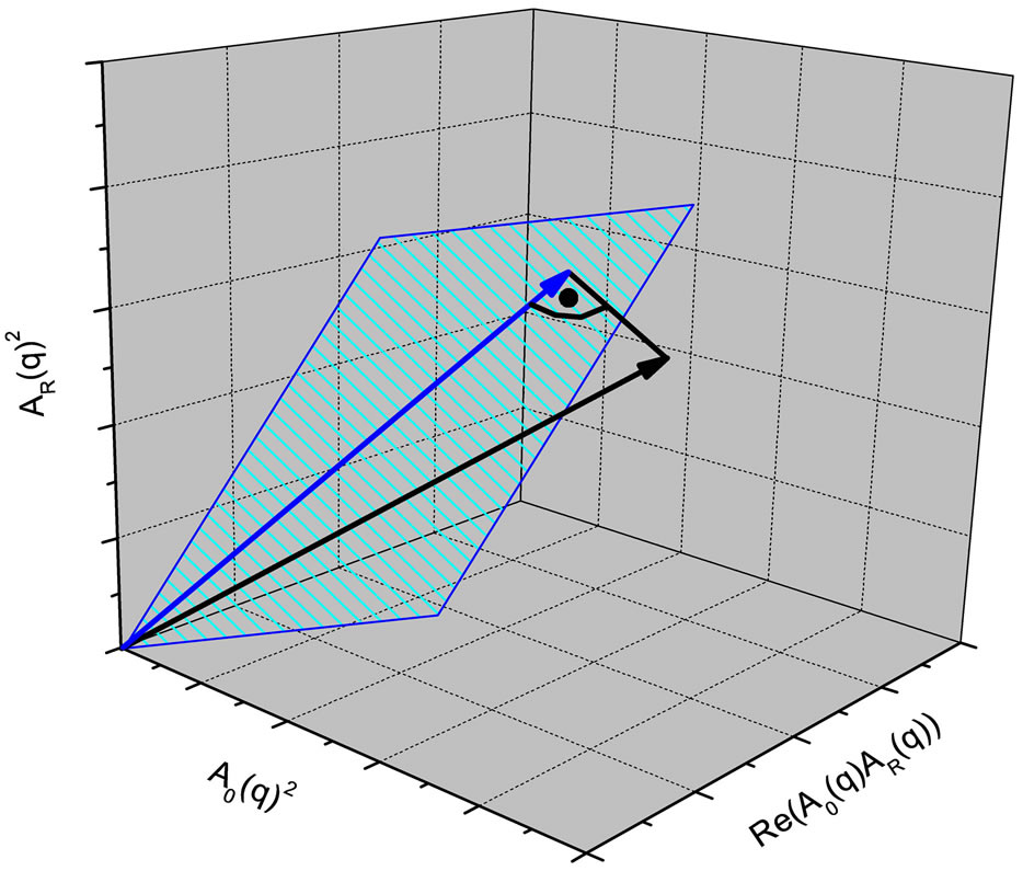
Figure 2. In analogy the blue plane represents the 3-dimensional hyper plane which is embedded in the 4-dimensional vector space. The possible solution vectors of the matrix equation are located in the plane. Due to measurement errors no solution vector of equation (24) exists, because the right hand vector is located outside of the plane (black vector). The approximate solution is the blue vector in the hyper plane with the shortest distance to the black vector.
the accuracy of the ASAXS sequence but require improved (!) accuracies [14,19].
2.4. The Eigenvector Problem in Anomalous Small-Angle X-Ray Scattering with More than Three Energies but at Different X-Ray Absorption Edges
In the following we will discuss the system of linear equations established by ASAXS measurements at different X-ray absorption edges such as binary alloys composed of components A and B, glasses or chemical solutions with different metal constituents.

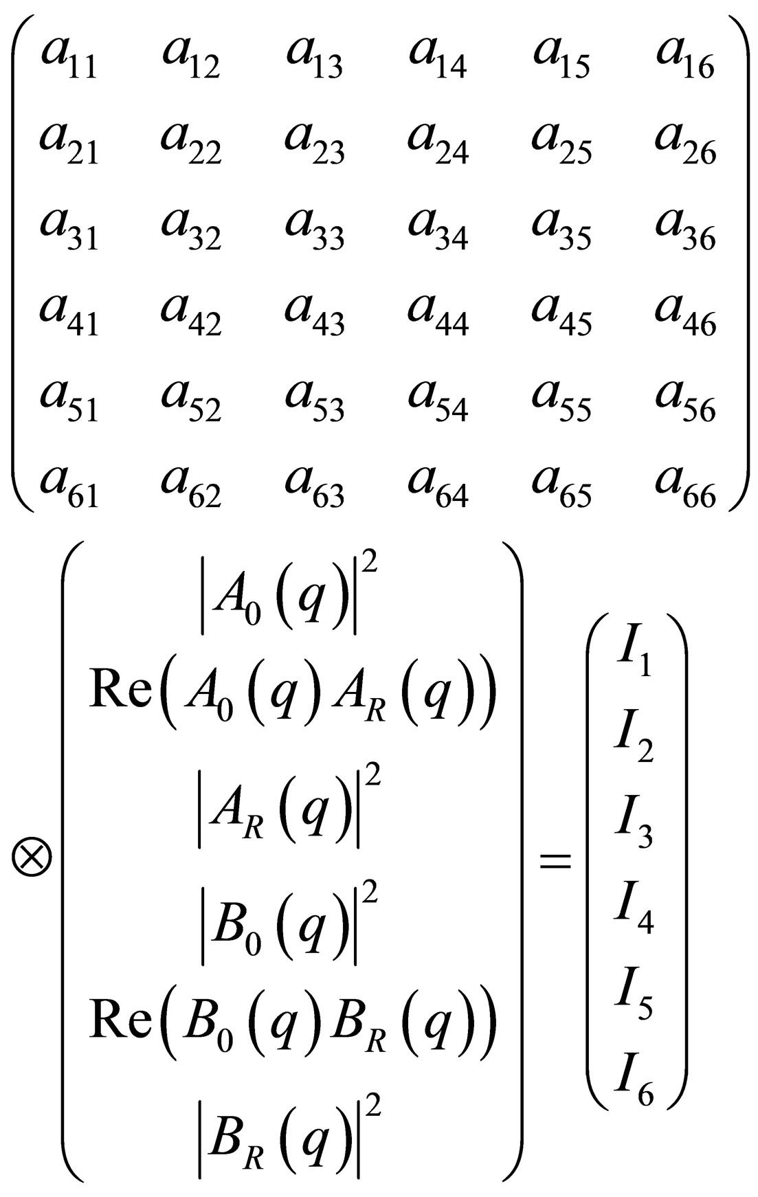 (25)
(25)
The Ii represent six scattering curves measured at different energies, three at energies of the 1st X-ray absorption edge, the other three at energies of the 2nd X-ray absorption edge. The aij again are functions of the density contrasts and the anomalous dispersion corrections of the different chemical constituents but this time from different X-ray absorption edges. The two X-ray absorption edges define two 3-dimensional vector spaces, which are orthogonal to each other i.e. the six linear equations are linear independent. Due to the different X-ray absorption edges the rank of the matrix is now six. Once again the triangular matrix can be found by elementary operation of the 6-dimensional vector equation, but for every subspace a triangular matrix can be established:
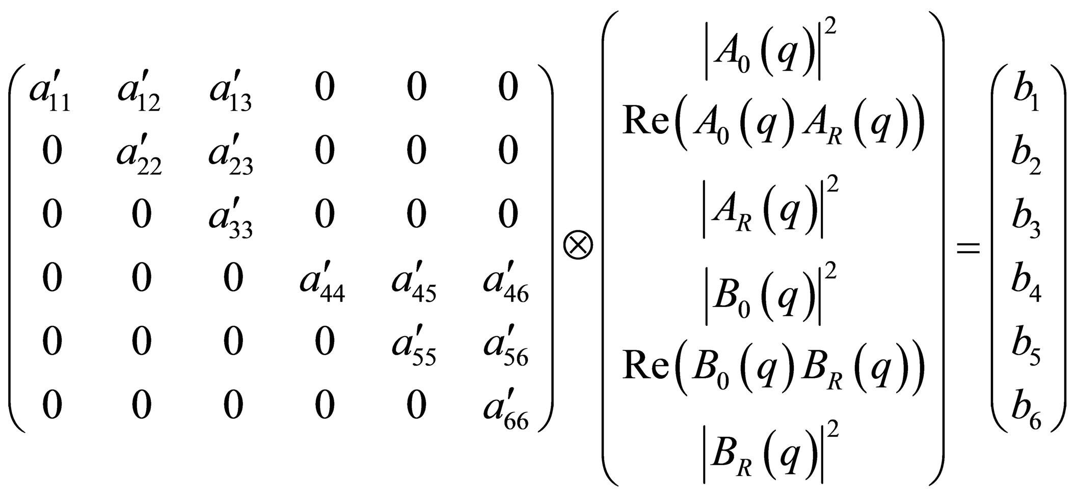 (26)
(26)
For the calculation of the eigenvalues, eigenvectors, pair correlation functions and the basic scattering functions the formula of the for-going chapter 2.2 can be used individually for each vector subspace (X-ray absorption edge). The eigenvectors in the 6-dimensional vector space are:
 (26a)
(26a)
The physical meaning of the 3 × 3-submatrix in Equation (26) filled with zero in the top right and bottom left is, that the atomic scattering factors of component B do not change, when tuning the energy at the X-ray absorption edge of component A and vice versa. The latter is a good approximation in the case, that the X-ray absorption edges lie far apart of each other. But of course there is a small change with energy and additionally, as in the forgoing chapter, there are measurement errors which enter the right hand vector. So a realistic formula of the vector equation is:
 (27)
(27)
If the matrix elements in the top right and bottom left matrix are small enough the eigenvector problem can be solved in good approximation separately for each absorption edge as outlined in chapter 2.2. In the case of contiguous X-ray absorption edges a more sophisticated equation must be employed for the solution of the eigenvector problem as is shown in Equation (28) for the example of a binary system:
 (28)
(28)
The same arguments hold for N X-ray absorption edges of condensed matter systems composed by N chemical components thereby establishing a 3N × 3N matrix in a 3N-dimensional vector space. If the N X-ray absorption edges lie far apart of each other the 3N-dimensional vector space is spanned by N 3-dimensional subspaces being orthogonal to each other in good approximation and the eigenvector problem can be solved separately in each 3-dimensional subspace via the formula of chapter 2.2. In the case of M < N contiguous X-ray edges the 3Ndimensional vector space is spanned by N − M 3-dimensional orthogonal subspaces and a 3M-dimensional subspace. The scheme of the vector equation is shown in Figure 3. Again the significance of the solution vectors obtained by these matrix inversions must be calculated via the Turing number [14].
As an example taken from a former publication Figure 4 depicts schematically the eigenvector representation in the 9-dimensional vector space of two ternary alloys (blue vectors) of different metallurgical states with the composition Ni68Nb16Y16 [10,11,14]. The light blue lines construct the foot points of the projection of the 9-dimensional vectors onto the three 3-dimensional subspaces of the three alloy components Nickel, Niobium and Yttrium. Because the X-ray absorption edges of the three elements
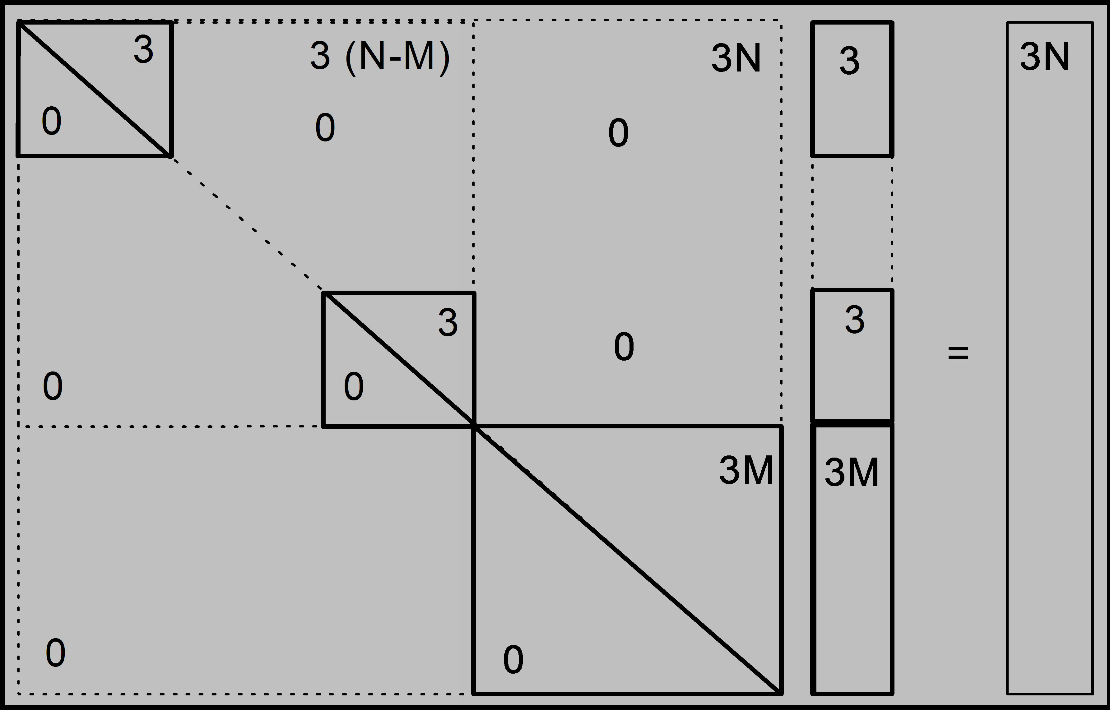
Figure 3. The vector equation established by a multi component system composed of N chemical elements. The small squares with the number 3 represent N-M 3 × 3 matrices in 3-dimensional subspaces. The small rectangles in the special solution vector represent the special 3-dimensional solution vector of Equation (6). The large square with the number 3M represents a 3M × 3M matrix of M chemical components with contiguous X-ray absorption edges. In the case of M = 2 it is the matrix of Equation (28). The subspaces are orthogonal to each other.
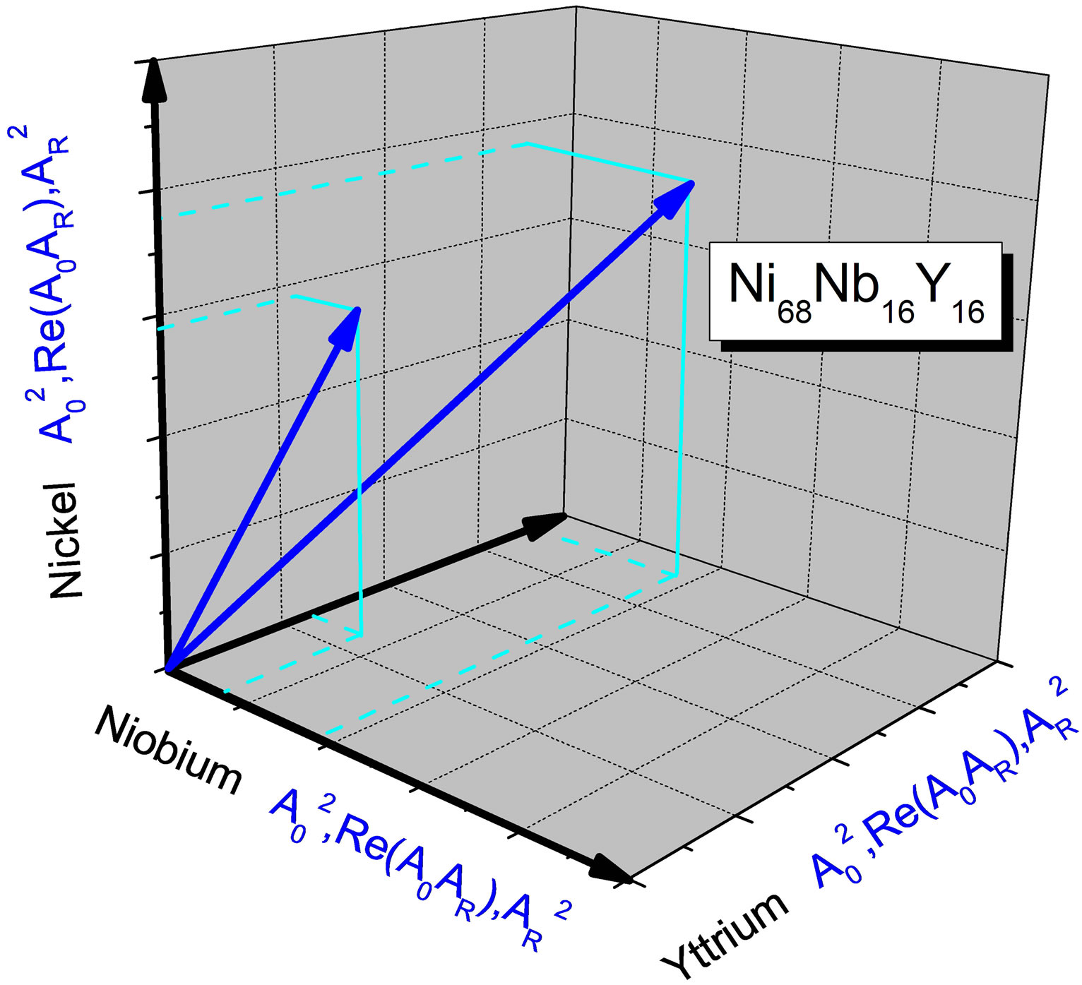
Figure 4. The blue vectors show the schematic eigenvector representation in the 9-dimensional vector space of two ternary alloys of different metallurgical states with the composition Ni68Nb16Y16 [10,11,14].
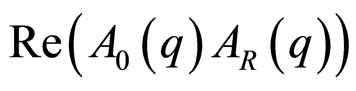
lie far apart of each other the three subspaces are orthogonal to each other in good approximation. Each subspace is spanned by the Cartesian orthogonal system of the pair correlation functions A02, Re(A0AR) and AR2 (see Figure 1). Thus within these three subspaces the pair correlation functions can be expressed in eigenvector representation i.e. each subspace provides the solution of the eigenvector problem independently from the other subspaces via the equations of chapter 2.2.
3. Conclusion
The mathematical basics of the system of linear equations established by Synchrotron radiation based Anomalous Small-Angle X-ray Scattering experiments have been analyzed. The linear algebraic theory provides the ASAXS techniques with five major improvements: (1) Analytical formula for the basic scattering functions, thereby omitting in-transparent fit or inversion procedures of unknown significance (2) a mathematical unambiguous solution of the system of linear equations by employment of the (linear) Gaussian elimination algorithm (3) an essential (but not sufficient) criterion (the Cauchy Schwarz inequality) allowing direct control, whether obtained basic scattering functions can possess significance or not and (4) a sufficient criterion represented by the Turing number, which tells directly the errors of the special solution vector facilitated by the inversion algorithm, thereby revealing its degree of significance. (5) The latter can be verified directly by ab initio error calculations, which start with the experimental errors entering the scattering curves of the ASAXS experiment (for instance the statistical errors obtained via single photon count techniques). For the calculation of the error propagation, the analytical formula is mandatory.
In summary, the eigenvector-based algorithm represents a superior mathematical description, because the problem is treated in the context of a linear matrix theory thereby offering the calculation of the significance of the solution, which cannot be provided by non-linear procedures. In other words, Linear Algebra gives deep insight (first intended by [20]) into ill-conditioned mathematical problems in condensed matter research thereby giving clear hints on how to overcome these problems by experimental and mathematical improvements. The subject underlines the crucial importance of Linear Algebra for search and understanding of mathematical algorithms in condensed matter research with Synchrotron radiation.
REFERENCES
- A. Guinier and G. Fournet, “Small-Angle Scattering of X-rays,” Wiley, New York, 1955.
- O. Glatter and O. Kratky, “Small-Angle X-Ray Scattering,” Academic Press, London, 1982.
- O. Kratky, “The World of Negligible Dimensions and Small Angle Diffraction of X-Rays and Neutrons on Biological Macromolecules,” Acta Leopoldina, Vol. 55, No. 256, 1983, pp. 6-72.
- G. Goerigk, R. Schweins, K. Huber and M. Ballauff, “The Distribution of Sr2+ Counterions around Polyacrylate Chains Analyzed by Anomalous Small-Angle X-Ray Scattering,” Europhysics Letters, Vol. 66, No. 3, 2004, pp. 331-337. http://dx.doi.org/10.1209/epl/i2003-10215-y
- G. Goerigk and D. L. Williamson, “Temperature Induced Differences in the Nanostructure of Hot-Wire Deposited Silicon-Germanium Alloys Analyzed by Anomalous SmallAngle X-Ray Scattering,” Journal of Applied Physics, Vol. 99, No. 8, 2006, Article ID: 084309. http://dx.doi.org/10.1063/1.2187088
- A. Bota, Z. Varga and G. Goerigk, “Biological Systems as Nanoreactors: Anomalous Small-Angle Scattering Study of the CdS Nanoparticle Formation in Multilamellar Vesicles,” The Journal of Physical Chemistry B, Vol. 111, No. 8, 2007, pp. 1911-1915. http://dx.doi.org/10.1021/jp067772n
- Z. Varga, A. Bota and G. Goerigk, “Localization of Dihalogenated Phenols in Vesicle Systems Determined by Contrast Variation X-ray Scattering,” Journal of Applied Crystallography, Vol. 40, No. 1, 2007, pp. 205-208. http://dx.doi.org/10.1107/S0021889807001987
- G. Goerigk, K. Huber and R. Schweins, “Probing the Extent of the Sr2+ Ion Condensation to Anionic Polyacrylate Coils: A Quantitative Anomalous Small-Angle X-Ray Scattering Study,” Journal of Chemical Physics, Vol. 127, No. 15, 2007, pp. 154908-1-154908-8. http://dx.doi.org/10.1063/1.2787008
- A. Bota, Z. Varga and G. Goerigk, “Structural Description of the Nickel Part of a Raney-Type Catalyst by Using Anomalous Small-Angle X-Ray Scattering,” The Journal of Physical Chemistry C, Vol. 112, No. 12, 2008, pp. 4427-4429. http://dx.doi.org/10.1021/jp800237b
- G. Goerigk and N. Mattern, “Critical Scattering of Ni– Nb–Y Metallic Glasses Probed by Quantitative Anomalous Small-Angle X-Ray Scattering,” Acta Materialia, Vol. 57, No. 12, 2009, pp. 3652-3661. http://dx.doi.org/10.1016/j.actamat.2009.04.028
- G. Goerigk and N. Mattern, “Spinodal Decomposition in Ni-Nb-Y Metallic Glasses Analyzed by Quantitative Anomalous Small-Angle X-Ray Scattering,” Journal of Physics: Conference Series, Vol. 247, 2010, Article ID: 012022. http://iopscience.iop.org/1742-6596/247/1/012022
- G. Goerigk, K. Huber, N. Mattern and D. L. Williamson, “Quantitative Anomalous Small-Angle X-Ray Scattering —The Determination of Chemical Concentrations in Nano-Scaled Phases,” European Physical Journal—Special Topics, Vol. 208, No. 1, 2012, pp. 259-274. http://dx.doi.org/10.1140/epjst/e2012-01623-2
- I. Akiba, A. Takechi, M. Sakou, M. Handa, Y. Shinohara, Y. Amemiya, N. Yagi and K. Sakurai, “Anomalous SmallAngle X-Ray Scattering Study of Structure of Polymer Micelles Having Bromines in Hydrophobic Core,” Macromolecules, Vol. 45, No. 15, 2012, pp. 6150-6157. http://dx.doi.org/10.1021/ma300461d
- G. Goerigk, “The Impact of the Turing Number on Quantitative ASAXS Measurements of Ternary Alloys,” JOM, Vol. 65, No. 1, 2013, pp. 44-53. http://dx.doi.org/10.1007/s11837-012-0451-9
- S. Lages, G. Goerigk and K. Huber, “SAXS and ASAXS on Dilute Sodium Polyacrylate Chains Decorated with Lead Ions,” Macromolecules, Vol. 46, No. 9, 2013, pp. 3570-3580. http://dx.doi.org/10.1021/ma400427d
- M. Sakou, A. Takechi, S. Murakami, K. Sakurai and I. Akiba, “Study of the Internal Structure of Polymer Micelles by Anomalous Small-Angle X-Ray Scattering at Two Edges,” Journal of Applied Crystallography, Vol. 46, No. 5, 2013, pp. 1407-1413. http://dx.doi.org/10.1107/S0021889813022450
- H. B. Stuhrmann, “Resonance Scattering in Macromolecular Structure Research,” Advances in Polymer Science, Vol. 67, 1985, pp. 123-163. http://dx.doi.org/10.1007/BFb0016608
- H. B. Stuhrmann, “Anomale Röntgenstreuung zur Erforschung makromolekularer Strukturen,” Macromolecular Chemistry, Vol. 183, No. 10, 1982, pp. 2501-2514. http://dx.doi.org/10.1002/macp.1982.021831020
- J. Westlake, “A Handbook of Numerical Matrix Inversion and Solution of Linear Equations,” Wiley, New York, 1968.
- J. P. Simon, O. Lyon and D. de Fontaine, “A Comparison of the Merits of Isotopic-substitution in Neutron SmallAngle Scattering and Anomalous X-Ray Scattering for the Evaluation of Partial Structure Functions in a Ternary Alloy,” Journal of Applied Crystallography, Vol. 18, 1985, pp. 230-236. http://dx.doi.org/10.1107/S0021889885010196
- D. T. Cromer and D. Liberman, Journal of Chemical Physics, Vol. 53, No. 5, 1970, pp. 1891-1898. http://dx.doi.org/10.1063/1.1674266
- D. T. Cromer and D. Liberman, Acta Crystallographica, Vol. A37, 1981, pp. 267-268.