Was Polchinski Wrong? Colombeau Distributional Rindler Space-Time with Distributional Levi-Cività Connection Induced Vacuum Dominance. Unruh Effect Revisited

doi:10.4236/jhepgc.2018.42023

Journal of High Energy Physics, Gravitation and Cosmology
Vol.04 No.02(2018), Article ID:84304,80 pages
10.4236/jhepgc.2018.42023

Jaykov Foukzon¹, Alexander Potapov², Elena Men’kova³

●How to Cite this Article

¹Center for Mathematical Sciences, Israel Institute of Technology, Haifa, Israel

²IRE RAS, Moscow, Russia

³All-Russian Research Institute for Optical and Physical Measurements, Moscow, Russia

This work is licensed under the Creative Commons Attribution International License (CC BY 4.0).

http://creativecommons.org/licenses/by/4.0/

Received: January 18, 2018; Accepted: April 27, 2018; Published: April 30, 2018

ABSTRACT

The vacuum energy density of free scalar quantum field $Φ$ in a Rindler distributional space-time with distributional Levi-Cività connection is considered. It has been widely believed that, except in very extreme situations, the influence of acceleration on quantum fields should amount to just small, sub-dominant contributions. Here we argue that this belief is wrong by showing that in a Rindler distributional background space-time with distributional Levi-Cività connection the vacuum energy of free quantum fields is forced, by the very same background distributional space-time such a Rindler distributional background space-time, to become dominant over any classical energy density component. This semiclassical gravity effect finds its roots in the singular behavior of quantum fields on a Rindler distributional space-times with distributional Levi-Cività connection. In particular we obtain that the vacuum fluctuations $〈 Φ^{2} 〉$ have a singular behavior at a Rindler horizon $δ_{R} = 0: 〈 Φ^{2} (δ) 〉 ≍ δ^{- 4}, δ ≍ c^{2} / a, a \to \infty$ . Therefore sufficiently strongly accelerated observer burns up near the Rindler horizon. Thus Polchinski’s account doesn’t violate the Einstein equivalence principle.

Keywords:

Vacuum Energy Density, Rindler Distributional Space-Time, Levi-Cività Connection, Semiclassical Gravity Effect, Einstein Equivalence Principle Space-Time, Levi-Cività Connection, Semiclassical Gravity Effect, Einstein Equivalence Principle

1. Introduction

In March 2012, Joseph Polchinski claimed that the following three statements cannot all be true [1] : 1) Hawking radiation is in a pure state, 2) the information carried by the radiation is emitted from the region near the horizon, with low energy effective field theory valid beyond some microscopic distance from the horizon, 3) the infalling observer encounters nothing unusual at the horizon. Joseph Polchinski argues that the most conservative resolution is: the infalling observer burns up at the horizon. In Polchinski’s account, quantum effects would turn the event horizon into a seething maelstrom of particles. Anyone who fell into it would hit a wall of fire and be burned to a crisp in an instant. As pointed out by physics community such firewalls would violate a foundational tenet of contemporary physics known as the equivalence principle, it states in part that an observer falling in a gravitational field―even the powerful one inside a black hole―will see exactly the same phenomena as an accelerated observer floating in empty space.

In this paper we argue that Polchinski was not wrong, but Unruh effect revision is needed.

1.1. What Is Colombeau Distributional Semi-Riemannian Geometry?

Recall that the classical Cartan’s structural equations show in a compact way the relation between a connection and its curvature, and reveal their geometric interpretation in terms of moving frames. In order to study the mathematical properties of singularities, we need to study the geometry of manifolds endowed on the tangent bundle with a symmetric bilinear form it is allowed to become degenerate (singular).

Remark 1.1.1. But if the fundamental tensor is allowed to be degenerate (singular), there are some obstructions in constructing the geometric objects normally associated to the fundamental tensor. Also, local orthonormal frames and coframes no longer exist, as well as the metric connection and its curvature operator [2] .

Remark 1.1.2. “Singular Semi-Riemannian Geometry”―the main brunch of contemporary semi-Riemannian geometry in which have been studied a smooth manifolds M furnished with a degenerate (singular) on a smooth submanifold $M^{'} ⊊ M$ metric tensor of arbitrary signature have been studied [2] .

Remark 1.1.3. In order to solve problems of the gravitational singularity in classical general relativity the singular semi-Riemannian geometry based on Colombeau calculas and Colombeau generalized functions was much developed, see [3] - [22] .

Remark 1.1.4. Let $G (M^{'})$ be algebra of Colombeau generalized functions on $M^{'} \subset M$ , let $\tilde{ℝ}$ be the ring of Colombeau generalized numbers [3] [4] [5] . Let ${(g_{ε})}_{ε}$ be Colombeau generalized metric tensor on M and let $R i c_{M^{'}} (p)$ be generalized Ricci tensor of the metric ${{(g_{ε} (p))}_{ε} |}_{M^{'}}$ [20] [21] . The main properties of such nonclassical manifolds with a degenerate (singular) metric tensor that is $R i c_{M^{'}} (p) \in G (M^{'}) \ C^{\infty} (M^{'})$ , i.e. for all $p \in M^{'} : R i c_{M^{'}} (p) \in \tilde{ℝ} \ ℝ$ .

Definition 1.1.1. Let $G (M^{'})$ be algebra of Colombeau generalized functions on $M^{'} \subset M$ , and let ${(g_{ε} (p))}_{ε}$ be Colombeau generalized metric tensor on M such that ${(g_{ε} (p))}_{ε}$ is the Colombeau solution of the Einstein field Equation (1.3.19), (see Remark 1.3.7). We define now the Colombeau distributional scalar curvature $R_{M} (p) = [{(R_{ε, M} (p))}_{ε}]$ (or distributional Ricci [20] [21] scalar) as the trace of $R i c_{M} (p) = [{(R i c_{ε, M} (p))}_{ε}]$ , i.e. $R_{M} (p) = t r [{(R i c_{ε, M} (p))}_{ε}]$ . Assume that $R_{M^{'}} (p) \in G (M^{'}) \ C^{\infty} (M^{'})$ .

Then we say that: (i) gravitational field ${(g_{ε} (p))}_{ε}$ (or corresponding distributional spacetime) has a gravitational singularity on a smooth compact submanifold $M_{c} \subset M$ iff $R_{M_{c}} (p) \in G (M_{c}) \ C^{\infty} (M_{c})$ ; (ii) gravitational field ${(g_{ε} (p))}_{ε}$ has a gravitational singularity with compact support iff $R_{M_{c}} (p) \in D^{'} (ℝ^{3})$ .

Remark 1.1.5. It turns out that the distributional Schwarzschild spacetime has a gravitational singularity with compact support at origin ${r = 0}$ [6] - [11] and at Schwarzschild horizon $S^{2} \times {r = 2 m}$ [18] [19] .

Definition 1.1.2. (i) Let $G (M)$ be algebra of Colombeau generalized functions on M, and let ${(g_{ε} (p))}_{ε}$ be Colombeau generalized metric tensor on M such that ${(g_{ε} (p))}_{ε}$ is the Colombeau solution of the generalized Einstein field Equation (1.3.19). The generalized point value of ${(g_{ε} (p))}_{ε}$ at generalized point ${((p_{ε}))}_{ε}$ is ${(g_{ε} (p_{ε}))}_{ε}$ . (ii) We define now the generalized point value of the distributional scalar curvature $R_{M} (p)$ at generalized point $p = [{((p_{ε}))}_{ε}]$ by formula $R_{M} (p) = [{(R_{ε, M} (p_{ε}))}_{ε}]$ .

1.2. Distributional Møller’s Geometry as Colombeau Extension of the Classical Moller’s Spacetime

As important example of Colombeau extension of the singular semi-Riemannian geometry mentioned above, we consider now Moller’s uniformly accelerated frame given by Moller’s line element [23] :

$d s^{2} = - {(a + g x)}^{2} d t^{2} + d x^{2} + d y^{2} + d z^{2} .$ (1.2.1)

Of couse Moller’s metric (1.2.1) degenerate at Moller horizon $x_{h o r}^{M o l} = - {(a / g)}^{- 1}$ . Note that formally corresponding to the metric (1.2.1) classical Levi-Civitá connection is [23]

$Γ_{44}^{1} (x) = (a + g x), Γ_{14}^{4} (x) = Γ_{41}^{4} (x) = \frac{1}{a + g x}$ (1.2.2)

and therefore classical Levi-Civit’a connection (1.2.2) of couse is not available at Moller horizon $x_{h o r}^{M o l} = - a \cdot g^{- 1}$ . Recall that fundamental tensor corresponding to the metric (1.2.1) was obtained in Moller’s paper [23] as a vacuum solution of the classical Einstein’s field equations

$G_{i}^{k} = R_{i}^{k} - \frac{1}{2} δ_{i}^{k} R = 0,$ (1.2.3)

where $R_{i}^{k}$ is the contracted Riemann-Christoffel tensor formally calculated by canonical way by using classical Levi-Civitá connection (1.2.2) and $R = R_{i}^{i}$ . Using Dingle’s formula [23] in case of the metric (1.2.1) we get

$\begin{array}{l} G_{2}^{2} (x) = G_{3}^{3} (x) = - \frac{1}{2 Δ (x)} {Δ^{″} (x) - \frac{{[Δ^{'} (x)]}^{2}}{2 Δ (x)}}, \\ Δ (x) = {(a + g x)}^{2}, \end{array}$ (1.2.4)

where $Δ^{'} (x) = \partial Δ (x) / \partial x$ and all other components of $G_{i}^{k}$ vanishes identically. Note that

$Δ^{'} (x) = 2 g (a + g x), Δ^{″} (x) = 2 g^{2} .$ (1.2.5)

Thus for any $x \neq - a \cdot g^{- 1}$ we get a classical result

$G_{2}^{2} (x) = G_{3}^{3} (x) = - \frac{1}{2 Δ (x)} {2 g^{2} - \frac{4 g^{2} {(a + g x)}^{2}}{2 Δ (x)}} \equiv 0.$ (1.2.6)

Let ${x_{n}}_{n \in ℕ}$ be a sequence such that $\lim_{n \to \infty} x_{n} = - a \cdot g^{- 1}, x_{n} \neq - a \cdot g^{- 1}, n \in ℕ$ . Then for any $n \in ℕ$ we get

$ℑ (x_{n}) = G_{2}^{2} (x_{n}) = G_{3}^{3} (x_{n}) = - \frac{1}{2 Δ (x_{n})} {2 g^{2} - \frac{4 g^{2} {(a + g x_{n})}^{2}}{2 Δ (x_{n})}} \equiv 0,$ (1.2.7)

and therefore $\lim_{n \to \infty} ℑ (x_{n}) \equiv 0$ . However

$\lim_{n \to \infty} Γ_{14}^{4} (x_{n}) = \underset{n \to \infty}{l i m} Γ_{41}^{4} (x_{n}) = \underset{n \to \infty}{l i m} \frac{1}{a + g x_{n}} = \infty,$ (1.2.8)

i.e. classical Levi-Civit’a connection given by (1.2.2) unavailable at Moller horizon.

Remark 1.2.1. In order to avoid difficultness mentioned above, we consider now the regularized Moller’s metric

$\begin{array}{l} d_{ε} s^{2} = - Δ_{ε} (x) d t^{2} + d x^{2} + d y^{2} + d z^{2}, \\ Δ_{ε} (x) = [{(a + g x)}^{2} + ε^{2}], ε \in (0, 1] . \end{array}$ (1.2.9)

Using now Dingle’s formula [23] for the case of (1.2.9) we get

$\begin{array}{l} ℑ (x; ε) = G_{2}^{2} (x; ε) = G_{3}^{3} (x; ε) = - \frac{1}{2 Δ_{ε} (x)} {{Δ^{″}}_{ε} (x) - \frac{{[{Δ^{'}}_{ε} (x)]}^{2}}{2 Δ_{ε} (x)}}, \\ Δ_{ε} (x) = [{(a + g x)}^{2} + ε^{2}] . \end{array}$ (1.2.10)

Note that

${Δ^{'}}_{ε} = 2 g (1 + g x), {Δ^{″}}_{ε} = 2 g^{2}$ (1.2.11)

and therefore

$\begin{matrix} ℑ (x; ε) = - \frac{1}{2 Δ_{ε} (x)} {2 g^{2} - \frac{2 g^{2} {(a + g x)}^{2}}{Δ_{ε} (x)}} \\ = - \frac{1}{2 Δ_{ε} (x)} {2 g^{2} - \frac{2 g^{2} [{(a + g x)}^{2} + ε^{2}] - 2 g^{2} ε^{2}}{Δ_{ε} (x)}} \\ = - \frac{g^{2} ε^{2}}{Δ_{ε}^{2} (x)} . \end{matrix}$ (1.2.12)

Remark 1.2.2. (i) Note that ${(ℑ (x; ε))}_{ε}, ε \in (0,1]$ is Colombeau generalized function such that

$c l [{(ℑ (x; ε))}_{ε}] \in G (ℝ)$ and $c l [{(ℑ (- {(a / g)}^{- 1}; ε))}_{ε}] = c l [{(ε^{- 2})}_{ε}] \in \tilde{ℝ} .$

Remark 1.2.3. Note that: (i) at any point $\tilde{x} \in \tilde{ℝ}$ such that $x \in ℝ$ and $x \neq - a \cdot g^{- 1}$ one obtains ${(ℑ (\tilde{x}; ε))}_{ε} \approx_{\tilde{ℝ}} \tilde{0}$ (see Definition 1.5.0 (i)) and therefore the Ricci tensor as well as the Ricci scalar are infinite small beyond Moller horizon $x_{h o r}^{M} = - \tilde{a \cdot g^{- 1}}$ . Thus at any point $\tilde{x}$ such that $x \in ℝ$ and $x \neq - a \cdot g^{- 1}$ we obtain the disered result in a good agriment with formall canonical calculation (see for example [24] , subsect. 2.1.6), (ii) obviously at any finite point $x_{f i n} \in \tilde{ℝ}$ (see Definition 1.5.0 (iii)) one obtains again ${(ℑ (\tilde{x}; ε))}_{ε} \approx_{\tilde{ℝ}} \tilde{0} .$

Remark 1.2.4. (I) Thus Colombeau generalized fundamental tensor ${(g_{i k} (ε))}_{ε}$ corresponding to Colombeau metric

$\begin{array}{l} (d_{ε} s^{2}) = - {(Δ_{ε} (x) d t^{2})}_{ε} + d x^{2} + d y^{2} + d z^{2}, \\ {(Δ_{ε} (x))}_{ε} = {([{(a + g x)}^{2} + ε^{2}])}_{ε}, ε \in (0,1] \end{array}$ (1.2.13)

that is non vacuum Colombeau solution (see [18] section 6 and [19] subsection 2.3 Distributional general relativity) of the Einstein’s field equations

(1.2.14)

For Rindler metric and we get

(1.2.15)

Definition 1.2.1. Distributional Moller’s geometry that is Colombeau extension of the classical Moller’s spacetime given by Colombeau generalized fundamental tensor (1.2.13).

1.3. Distributional Schwarzschild Geometry as Colombeau Extension of the Classical Singular Schwarzschild Spacetime

1.3.1. Colombeau Extension of the Classical Singular Schwarzschild Spacetime Furnished with a Degenerate and Singular Schwarzschild Metric

As another important example of Colombeau extension of the singular semi-Riemannian geometry we consider now classical singular Schwarzschild spacetime furnished with a degenerate and singular Schwarzschild metric

(1.3.1)

Remark 1.3.1. Note that formally corresponding to the metric (1.3.1) classical Levi-Civitá connection given by canonical Christoffel symbols are [24] :

(1.3.2)

i.e. classical Levi-Civita connection given by Equation (1.3.2) unavailable at Schwarzschild horizon.

Remark 1.3.2. Nevertheless in classical handbooks [24] - [37] were mistakenly assumed that classical semi-Riemannian geometry holds on whole Schwarzschild manifold and therefore canonical formal calculation gives

(1.3.3)

By Equation (1.3.2) it is mistakenly pointed out that the Schwarzschild metric has only a coordinate singularity at and there is no gravitational singularity at Schwarzschild horizon.

Remark 1.3.3. Note that canonical formal calculation gives

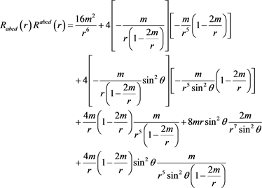(1.3.4)

Assume that and, i.e.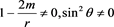, then from

Equation (1.3.4) one obtains directly

(1.3.5)

Remark 1.3.4. Notice that: if then RHS of the Equation (1.3.4) become uncertainty

(1.3.6)

A. Einstein emphasized that uncertainty of the form 0/0 mentioned above that is a fundamental mathematical problem, see [38] , p. 74. However in order to avoid this difficulty mentioned above in physical literature [24] - [37] one mistakenly defines

(1.3.7)

However Equation (1.3.7) doesn’t holds at because classical Levi-Civitá connection (1.3.2) of course is not available at Schwarzschild horizon, see Remark 1.3.1.

Remark 1.3.5. Thus from Equation (1.3.4) for and we get

(1.3.8)

and we get nothing at Schwarzschild horizon. Therefore semi-Riemannian geometry break down at Schwarzschild horizon [18] [19] .

Remark 1.3.6. Recall that canonical derivation of the canonical singular Schwarzschild metric in classical handbooks is always based on assumption that:

Assumption 1.3.1. Classical semi-Riemannian geometry holds on the whole semi-Riemannian manifold, see for example [26] .

Let be the metric

(1.3.9)

where as. Then under Assumption 1.3.1 one obtains [26] :

(i) all are zero except

(1.3.10)

The equations are

(1.3.11)

and

(1.3.12)

and

(1.3.13)

From Equation (1.3.11)-Equation (1.3.12) one obtains

(1.3.14)

Therefore AB = constant. Since at we have and one obtains. From Equation (1.3.13)-Equation (1.3.14) one obtains

(1.3.15)

and by integration Equation (1.3.15) one obtains, where is an integration constant. Finally one obtains well known classical result

(1.3.16)

From Equation (1.3.16) and consideration above (see Remark 1.3.4) Assumption 1.3.1 wrong, otherwise one obtains the contradiction.

Remark 1.3.7. In order to avoid this difficulty:

(i) we have introduced instead a classical Einstein field equations

(1.3.17)

[where the sign of the energy-momentum tensor is defined by (is the energy density)]

(1.3.18)

apropriate Colombeau generalization of the Equation (1.3.17)-Equation (1.3.18) such that

(1.3.19)

where the sign of the distributional energy-momentum tensor is defined by

(1.3.20)

see [18] [19] .

(ii) we have introduced instead of Assumption 1.3.1 the following assumption.

Assumption 1.3.2. Distributional semi-Riemannian geometry holds on the whole distributional semi-Riemannian manifold.

Definition 1.3.1. Let and the regularization of the functions and [defined above by Equation (1.3.16)] such that the following conditions are satisfied:

(i) and are Colombeau generalized functions;

(ii) (1.3.21)

(iii)

(iv)

Let be the Colombeau metric

(1.3.22)

and let be the distributional Levi-Civita connection [18] [19] corresponding to Colombeau metric (1.3.22). Then under Assumption 1.3.2 one obtains:

(i) all are zero except

(1.3.23)

(1.3.24)

and

(1.3.25)

and

(1.3.26)

Weak distributional limit in of the RHS of the Equation (1.3.18), i.e. is calculated in our papers [18] [19] , see also Appendix B.

Remark 1.3.8. It turns out that the distributional Schwarzschild metric (1.3.22) has a gravitational singularity with compact support at origin [6] - [11] and at Schwarzschild horizon [18] [19] .

1.3.2. Colombeau Extension of the Schwarzschild Spacetime in Isotropic Coordinates

Let us consider now nonclassical spacetime furnished with a degenerate at horizon but nonsingular (at horizon) metric and known in physical literature as Schwarzschild spacetime in isotropic coordinates [24] :

(1.3.27)

Nonsingular metric (1.3.27) is obtained by the coordinate transformation:, between the Schwarzschild radial coordinate r and the isotropic radial coordinate. Under formal calculation one obtains [24] :

(1.3.28)

i.e. classical Levi-Civitá connection given by (1.3.28) of course unavaluble at horizon. However in physical literature under ubnormal calculation it was mistakenly pointed out that the Ricci tensor and the Ricci scalar vanish identically and Kretschman scalar is

(1.3.29)

Remark 1.3.9. In order to avoid difficulty with the degeneracy of the metric (1.3.27) mentioned above, we consider now the corresponding distributional Colombeau metric which reads

(1.3.30)

where.

Definition 1.3.2. Distributional Schwarzschild geometry in isotropic coordinates which is Colombeau extension of the classical spacetime (1.3.27), given by Colombeau generalized fundamental tensor (1.3.30).

Colombeau generalized metric (1.3.30) nondegenerate at horizon in Colombeau sence and distributional Levi-Civitá connection now available on the whole distributional Schwarzschild spacetime in isotropic coordinates. Notice that generalized metric (1.3.30) has the form given by Equation (A.1) (see Appendix A) with

(1.3.31)

From Equation (A.2) (see Apendix A2) and Equation (1.3.31) in the limit, we get

(1.3.32)

Compare the equation with Equation (1.2.12).

Remark 1.3.10. Notice that in contrast with result of naive formal calculation mentioned above (see Equation (1.3.29)) we get:

(i)

(ii)

(iii)

1.4. On the Near Horizon Colombeau Approximation for the Classical Singular Schwarzschild Black Hole Geometry

Let us perform the following coordinate transformation

(1.4.1)

to the classical singular Schwarzschild metric

(1.4.2)

we get

(1.4.3)

In Equation (1.4.2), m is the central mass, and. Taking the limit, the spherical horizon becomes planar and Equation (1.4.3) leads to the Colombeau type metric

(1.4.4)

which is distributional Rindler’s spacetime if we neglect the angular contribution. The condition is equivalent to the “near horizon approximation” for the exterior geometry of a black hole: for the line element (1.4.2) appears, indeed, as

(1.4.5)

By using simple coordinate transformations it could be shown that (1.4.5) again becomes the distributional Rindler metric when we take or and are negligible. We stress that the condition only is not enough to obtain Rindler’s spacetime which has no spherical symmetry as Schwarzschild.

Remark 1.4.1. At this stage of consideration, it is already clear that near horizon Schwarzschild black hole geometry has a gravitational singularity at horizon. Notice that in classical literature (see, for example, [24] - [36] ) near horizon Schwarzschild black hole geometry were mistakenly accepted as regular with the Ricci tensor and the Ricci scalar vanish identically.

1.5. Colombeau Distributional Semi-Riemannian Geometry. Preliminaries

1.5.1. The Ring of Colombeau Generalized Numbers

Designation 1.5.1. We denote by the ring of real, Colombeau generalized numbers. Recall that [2] [3] by definition

where

(1.5.0)

Designation 1.5.2. In the sequel we denote by:

, where an open subset of, the algebra of all the sequences (for short,) of smooth functions.

is the differential subalgebra of the elements such that for all, for all there exists with the following property: as.

the differential subalgebra of the elements such that for all, for all and the following property holds: as.

Definition 1.5.1. The elements of and are called moderate and negligible, respectively.The factor algebra

(1.5.1)

is the algebra of Colombeau generalized functions on.

Remark 1.5.0. Note that: (i) there exists natural embedding such that for all, , , for all, (ii) the ring can be endowed with the structure of a partially ordered ring: for, if and only if there are representatives and with for all.

Definition 1.5.2. (i) Let. We say that is infinite small Colombeau generalized number and abbraviate

or, if there exists representative and some such that, as. We abbraviate iff.

(ii) We say that is infinite large Colombeau generalized number and abbraviate

if.

(iii) We say that is finite Colombeau generalized number and abbraviate if there are such that.

Definition 1.5.3. Let and be a set

correspondingly. We introduce equivalence relation given by

and denote by the set of generalized points. Moreover, if is the class of in then the set of compactly generalized points is

Note that if the -property holds for one representative of then it holds for every representative. Also, for we have that the factor is the usual algebra of real generalized numbers.

Definition 1.5.4. We denote by and the set of inite large and infite small generalized points correspondingly. It is clear that the generalized point value of at is

Definition 1.5.5. Let be infinite small Colombeau generalized number with representative. We introduce a norm of such representative by formula.

1.5.2. A Real Colombeau Vector Bundle

Definition 1.5.6. A real vector bundle consists of:

1) Topological spaces X (base space) and E (total space)

2) A continuous surjection (bundle projection)

3) For every x in X, the structure of a finite-dimensional vector space over Colombeau ring on the fiber where the following compatibility condition is satisfied: for every point in X, there is an open neighborhood U, a natural number k, and a homeomorphism

such that for all, for all vectors v in, and the map is a linear isomorphism between the vector spaces and.

The open neighborhood U together with the homeomorphism is called a local trivialization of the Colombeau vector bundle. The local trivialization shows that locally the map “looks like” the projection of on U.

The Cartesian product, equipped with the projection, is called the trivial bundle of rank k over X.

1.5.3. The Algebra of Colombeau Generalized Functions

The basic idea of Colombeau’s theory of generalized functions is a regularization by sequences (nets) of smooth functions and the use of asymptotic estimates in terms of a regularization parameter. Let with for all (M a separable, smooth orientable Hausdorff manifold of dimension n).The algebra of Colombeau generalized functions on M is defined as the quotient

(1.5.2)

of the space of sequences of moderate growth modulo the space of negligible sequences. More precisely the notions of moderateness resp. negligibility are defined by the following asymptotic estimates (or denoting the space of smooth vector fields on M).

(1.5.3)

Elements of are denoted by

(1.5.4)

With componentwise operations is a fine sheaf of differential algebras with respect to the Lie derivative defined by

(1.5.5)

The spaces of moderate resp. negligible sequences and hence the algebra itself may be characterized locally, i.e., Î iff for all charts, where on the open set in the respective estimates Lie derivatives are replaced by partial derivatives. Smooth functions are embedded into simply by the “constant” embedding, i.e., , hence is a faithful subalgebra of. On open sets of compactly supported distributions are embedded into G via convolution with a mollifier with unit integral satisfying for all; more precisely setting we have. In case is not compact one uses a sheaf-theoretical construction.

1.5.4. Colombeau Tangent Vector

Let, where is a differentiable function and let v be a vector in. We define the Colombeau directional derivative in the v direction at a point by

(1.5.6)

The Colombeau tangent vector at the point x may then be defined as

(1.5.7)

Let, where be differentiable functions, let be tangent vectors in at and let. Then

1.5.5. Colombeau Tangent Vector to Differentiable Manifold M

Let M be a differentiable manifold and let be the algebra of real-valued Colombeau generalized functions on M. Then the tangent vector to M at a point x in the manifold is given by the derivation which shall be linear―i.e., for any and we have

Note that the derivation will by definition have the Leibniz property

1.5.6. Colombeau Vector Fields on Distributional Manifolds

Colombeau vector field (denoted often by) on a manifold M is a linear map:

such that for all:

(1.5.8)

1.5.7. Colombeau Tangent Space

Suppose now that M is a manifold. A real-valued Colombeau generalized function is said to belong to if and only if for every coordinate chart, the map is infinitely differentiable. Note that is a real associative algebra with respect to the pointwise product and sum of Colombeau generalized functions. Pick a point. A derivation at x is defined as a linear map that satisfies the Leibniz identity:

which is modeled on the product rule of calculus.

If we define addition and scalar multiplication on the set of derivations at x by

and

where, then we obtain a real vector space over, which we define as the Colombeau tangent space of M at x.

1.5.8. Colombeau Dual Space

Given any vector space over Colombeau algebra, the (algebraic) Colombeau dual space (also denoted for a short by) is defined as the set of all linear maps. Since linear maps are vector space homomorphisms, the Colombeau dual space is also sometimes denoted by. The Colombeau dual space itself becomes a vector space over when equipped with an addition and scalar multiplication satisfying: (i) and (ii), where .

1.5.9. Colombeau Cotangent Space

Let M be a smooth manifold and let x be a point in M. Let be Colombeau tangent space at x. Then Colombeau cotangent space at x is defined as the Colombeau dual space of.

Suppose now that M is a manifold and let. The differential of at a point x is the map: where is a tangent vector at x, thought of as a derivation. In either case, is a linear map on and hence it is a tangent covector at x.

We can then define the differential map at a point x as the map which sends to. Properties of the differential map include:

(i) for, (ii).

Let for any be a smooth map of smooth manifolds. Given some, the Colombeau differential of at x is a linear map from Colombeau tangent space of M at x to Colombeau tangent space of N at. The application of to a tangent vector X is called the pushforward of X by.

1.5.10. -Module of Generalized Sections of a Vector Bundle

The -module of generalized sections of a vector bundle and in particular the space of generalized tensor fields is defined along the same lines using analogous asymptotic estimates with respect to the norm induced by any Riemannian metric on the respective fibers. We denote generalized sections by. Alternatively we may describe a section by a family, where is called the local expression of S with its components (a vector bundle atlas and , with N denoting the dimension of the fibers) satisfying for all, where denotes the transition functions of the bundle.

Remark 1.5.1. Smooth sections of again may be embedded as constant nets, i.e.,

Since is a subring of also may be viewed as -module and the two respective module structures are compatible with respect to the embeddings.

Moreover we have the following algebraic characterization of the space of generalized sections

(1.5.9)

where denotes the space of smooth sections and the tensor product is taken over the module. Generalized tensor fields may be viewed likewise as -resp. -multilinear mappings, i.e., as -resp. -modules we have

(1.5.10)

Here resp. denotes the space of smooth vector resp. covector fields on M.

1.5.11. Generalized Pseudo-Riemannian Manifold

A generalized tensor field is called a generalized Pseudo-Riemannian metric if it has a representative satisfying

(i) is a smooth Pseudo-Riemannian metric for all, and

(ii) is strictly nonzero on compact sets, i.e.,

We call a separable, smooth Hausdorff manifold M furnished with a generalized pseudo-Riemannian metric generalized pseudo-Riemannian manifold or generalized spacetime and denote it by. The action of the metric on a pair of generalized vector fields will be denoted by or [20] [21] .

A generalized metric is non-degenerate in the following sense:

(1.5.11)

Note that condition (ii) above is precisely equivalent to invertibility of in the generalized sense.

The inverse metric is a well defined element of, depending exclusively on (i.e., independent of the particular representative).

Moreover if, where g is a classical -pseudo-Riemannian metric then.

From now on we denote the inverse metric by, its components by and the components of a representative by. Also we shall denote the generalized metric by and its representative by and use summation convention.

Notice that induces a -linear isomorphism by, which as in the classical context extends naturally to generalized tensor fields of all types.

1.5.12. Colombeau Isometric Embedding

Let and be generalized pseudo-Riemannian manifolds. An isometric Colombeau embedding is a Colombeau generalized function: which preserves the metric in the sense that is equal to the pullback of by, i.e.. Explicitly, for any two tangent vectors we have.

1.5.13. Generalized Connection on a Generalized Pseudo-Riemannian Manifold

Generalized connection on a manifold M is a map satisfying:

(D1) is -linear in.

(D2) is -linear in.

(D3) for all.

Let be a chart on M with coordinates xⁱ. The generalized Christoffel symbols for this chart are given by the generalized functions defined by

(1.5.12)

Theorem. [21] . (I) Let be a generalized pseudo-Riemannian manifold. Then there exists a unique generalized connection such that

(D4) and

(D5)

hold for all in.

is called generalized Levi-Civita connection of M and characterized by the so-called Koszul formula

(1.5.13)

(II) On every chart we have for the generalized Levi-Civita connection of and any vector field

(1.5.14)

The generalized Christoffel symbols are given by

(1.5.15)

or by using representative

(1.5.16)

We define now the action of a classical (smooth) connection D on generalized vector fields and by

(III) Let be a generalized pseudo-Riemannian manifold.

(i) If where is a classical smooth metric then we have,in any chart, (with denoting the Christoffel Symbols of). Hence for all:

(ii) If, where a classical smooth metric, and, or, , then.

(iii) Let, where a classical -metric, then, in any chart,. If in addition, , and then

1.5.14. The Generalized Riemannian Curvature Tensor

Let be a generalized pseudo-Riemannian manifold with a generalized Levi-Civita connection.

(i) The generalized Riemannian curvature tensor is defined by

(1.5.17)

(ii) The generalized Ricci curvature tensor is defined by

(1.5.18)

(iii) The generalized Ricci scalar is defined by

(1.5.19)

(iv) Finally we define the generalized Einstein tensor by

(1.5.20)

1.6. Super Generalized Functions

1.6.1. The Nonsmooth Regularization via Horizon

Examining now the Schwarzschild metric (1.3.1) (note that the origin is now excluded from our considerations, the space we are working on is) in a neighborhood of the horizon, we see that, whereas is smooth, is not even. Thus, regularizing the Schwarzschild metric amounts to embedding into, for example as that given in paper [17] , one obtains Colombeau generalized metric

(1.6.1)

Here and is a mollifier.

Obviously, (1.6.1) is degenerate at, because is zero at the horizon. Due to the degeneracy of (33), the Levi-Civitá connection is not available. In order avoid this difficultness in literature the following generalized pseudo-connection was considered [17] :

(1.6.2)

Obviously the generalized pseudo-connection coincides with the classical Levi-Civitá connection on since, there. However the generalized pseudo-connection is not a true generalized Levi-Civitá connection on since does not respect the Colombeau generalized metric (1.6.1), i.e., , e.g., . Compatibility with the metric is a priori ruled out by the following statement: there exists no connection whatsoever under which would be a parallel tensor. However in a weak sense, the connection (1.6.2) is metric compatible:. In additional [17] :

(1.6.3)

where is a Ricci tensor corresponding to generalized pseudo-connection (1.6.2), and therefore Colombeau object viewed as a classical distribution on gives

(1.6.4)

Remark 1.6.1. In paper [17] the equality (1.6.4) mistakenly considered as a proof that the metric singularity at the Schwarzschild horizon is only a coordinate singularity.

Remark 1.6.2. Due to the degeneracy of any smooth regularization of the metric (1.3.1) no canonical Levi-Civitá connection could be defined. In order to avoid such difficultnes in our papers [18] [19] the nonsmooth regularization via horizon is considered, see Section 2 below. However such regularization demands appropriate extension of the Colombeau algebra.

1.6.2. The Super Generalized Functions

The basic idea of the theory of super generalized functions is regularization by sequences (nets) of appropriate classes of non smooth and discontinuous functions or classical distributions and the use of asymptotic estimates in terms of a regularization parameter. Let with for all (M a separable, smooth orientable Hausdorff manifold of dimension n). Such sequences are called super generalized functions. The algebra of super generalized functions on M is defined as the quotient

(1.6.5)

(1.6.6)

Here denoting the weak Lie derivative in L.Schwartz sense and where Landau symbol appears, having the following meaning:

We denote by the ring of real, Colombeau super generalized numbers., where

(1.6.7)

Let with for all (M a separable, smooth orientable Hausdorff manifold of dimension n). By using canonical imbeding the algebra of Colombeau super generalized functions on M is defined also in the equivalent form as the quotient

(1.6.8)

(1.6.9)

The -module of super generalized sections of a vector bundle and in particular the space of super generalized tensor fields is defined along the same lines using analogous asymptotic estimates with respect to the norm induced by any Riemannian metric on the respective fibers. We denote super generalized sections by

. Alternatively we may describe a section

by a family, where is called the local expression of S with its components

(a vector bundle atlas and, with N denoting the

dimension of the fibers) satisfying for all where denotes the transition functions of the bundle.

Remark 1.6.3. Smooth sections of again may be embedded as constant nets, i.e.,

Since is a subring of also may be viewed as -module and the two respective module structures are compatible with respect to the embeddings.

Moreover we have the following algebraic characterization of the space of super generalized sections

(1.6.10)

(1.6.11)

Here resp. denotes the space of smooth vector resp. covector fields on M.

1.6.3. Super Generalized Pseudo-Riemannian Manifold

A super generalized tensor field is called a super generalized Pseudo-Riemannian metric if it has a representative satisfying:

(i) is a smooth Pseudo-Riemannian metric for all, and

(ii) is strictly nonzero on compact sets, i.e.,

We call a separable, smooth Hausdorff manifold M furnished with a super generalized pseudo-Riemannian metric super generalized pseudo-Riemannian manifold or super generalized spacetime and denote it by. The action of the metric on a pair of super generalized vector fields will be denoted by or.

A super generalized metric is non-degenerate in the following sense:

(1.6.12)

Note that condition (ii) above is precisely equivalent to invertibility of in the super generalized sense. The inverse metric is a well defined element of, depending exclusively on (i.e., independent of the particular representative). Moreover if, where is a classical -pseudo-Riemannian metric then. From now on we denote the inverse metric by, its components by and the components of a representative by. Also we shall denote the super generalized metric by and its representative by and use summation convention.Notice that induces a -linear isomorphism by , which as in the classical context extends naturally to generalized tensor fields of all types.

Let and be super generalized pseudo-Riemannian manifolds. An isometric Colombeau embedding is a Colombeau super generalized function which preserves the metric in the sense that is equal to the pullback of by, i.e.. Explicitly, for any two tangent vectors we have .

1.6.4. Super Generalized Connection on a Super Generalized Pseudo-Riemannian Manifold

Super generalized connection on a manifold M is a map satisfying:

(D1) is -linear in.

(D2) is -linear in.

(D3) for all.

Let be a chart on M with coordinates. The super generalized Christoffel symbols for this chart are given by the super generalized functions defined by

(1.6.13)

Theorem. (I) Let be a super generalized pseudo-Riemannian manifold. Then there exists a unique super generalized connection such that

(D4) and

(D5)

hold for all in.

is called super generalized Levi-Civita connection of M and characterized by the so-called Koszul formula

(1.6.14)

(II) On every chart we have for the super generalized Levi-Civita connection of and any vector field

(1.6.15)

The super generalized Christoffel symbols are given by

(1.6.16)

or by using representative

(1.6.17)

We define now the action of a classical (smooth) connection D on super generalized vector fields and by

(III) Let be a super generalized pseudo-Riemannian manifold.

(i) If where is a classical smooth metric then we have,in any chart, (with denoting the Christoffel Symbols of). Hence for all.

(ii) If, where a classical smooth metric, and, or, , then.

(iii) Let, where a classical -metric, then, in any chart,. If in addition , , and then.

1.6.5. The Super Generalized Riemannian Curvature Tensor

Let be a super generalized pseudo-Riemannian manifold with a super generalized Levi-Civita connection.

(i) The super generalized Riemannian curvature tensor is defined by

(1.6.18)

(i) The super generalized Ricci curvature tensor is defined by

(1.6.19)

(iii) The super generalized Ricci scalar is defined by

(1.6.20)

4) Finally we define the super generalized Einstein tensor by

(1.6.21)

2. Distributional Schwarzschild Geometry by Using Nonsmooth Regularization via Horizon

2.1. Distributional Schwarzschild Spacetime as Colombeau Extension of the Lorentzian Manifold with Nonregularity Conditions on Schwarzschild Horizon

Singular space-times present one of the major challenges in general relativity. Originally it was believed that their singular nature is due to the high degree of symmetry of the well-known examples ranging from the Schwarzschild geometry to the Friedmann-Robertson-Walker cosmological models. However, Penrose and Hawking [36] have shown in their classical singularity theorems that singularities are a phenomenon which is inherent to general relativity. Since the standard approach allows only smooth space-time metrics, one has to exclude the so called singular regions from the space-time manifold. In a recent work many authors advocated the use Colombeau distributional techniques [5] - [22] to calculate the energy-momentum tensor of the Schwarzschild geometry. It turns out that it is possible to include the singular region (i.e. the space-like line with respect to Schwarzschild coordinates) in the space-time which now no longer is a vacuum geometry, and to identify it with the support of the energy-momentum tensor [5] [9] [11] [12] [13] . The same “physically expected” result for the distributional energy momentum tensor of the Schwarzschild geometry was obtained in papers [12] - [22] , i.e.,

(2.1.1)

in a conceptually satisfactory way.

Remark 2.1.1. The result (2.1.1) can be easily obtained by using apropriate nonsmooth regularization of the Schwarzschild singularity at the origin.

The nonsmooth regularization of the Schwarzschild singularity at the origin was originally considered by N. R. Pantoja and H. Rago in paper [12] . Such non smooth regularization of the Schwarzschild singularity is

(2.1.2)

Here is the generalized Heaviside function,where

(2.1.3)

and the limit is understood in a weak distributional sense. The equation

(2.1.4)

with, as given in (2.1.4) can be considered as Colombeau version of the Schwarzschild line element in curvature coordinates. From Equation (2.1.2), the calculation of the distributional Einstein tensor, , , proceeds in a straighforward manner. By simple calculation one obtains [12] :

(2.1.5)

and

(2.1.6)

In papers [10] [27] Colombeau distributional techniques were extended to the general axisymmetric, stationary Kerr and Newman space-time family. This family also contains the Schwarzschild geometry and its charged extension the Reissner-Nordstrø m solution as special cases of spherical symmetry. In the paper [22] it was shown that the solutions will satisfy the Einstein equations everywhere if the energy-momentum tensor has an appropriate singular addition of nonelectromagnetic origin. When this addition term is included, the total energy turns out to be finite and equal to, while the angular momentum for the Kerr and Kerr-Newman solutions is.

Remark 2.1.2. The nonsmooth regularization of the Schwarzschild singularity above the horizon is

(2.1.7)

Here is the generalized Heaviside function and the limit is understood in a weak distributional sense. The equation

(2.1.8)

, as given in (2.1.8) can be considered as Colombeau version of the Schwarzschild line element in curvature coordinates above horizon. From Equation (2.1.7), the calculation of the distributional Einstein tensor above horizon, , , proceeds in a straighforward manner. By simple calculation one obtains

(2.1.9)

The truncated distributional Schwarzschild geometry.

There exist two different types of distributional Schwarzschild blackhole geometry corresponding to classical Schwarzschild solution. That is: (i) full distributional Schwarzschild blackhole geometry, given by Colombeau generalized object, for example by Equation (1.3.30), see Figure 1(a) and (ii) the truncated distributional Schwarzschild space-time given by Colombeau generalized object (2.1.7)-(2.1.8), i.e. in this case distributional spacetime ends just on the Schwarzschild horizon, see Figure 1(b).

Remark 2.1.3. In a nutshell, there is a widespread but mistaken belief that there exist true gravitational singularities, for example at origin of the

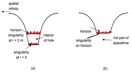
Figure 1. (a) The picture of a distributional Schwarzschild blackhole, given by Colombeau generalized object (1.3.30). Distributional spacetime ends just on the Schwarzschild singularity. (b) The truncated Schwarzschild distributional geometry, given by Colombeau generalized object (2.1.7)-(2.1.8). Distributional spacetime ends just on the Schwarzschild horizon.

Schwarzschild spacetime, and non principal and non gravitational, i.e. purely coordinate singularities, for example at horizon of the Schwarzschild spacetime. A coordinate singularity or coordinate degeneracy occurs when an apparent singularity or degeneracy occurs in one coordinate frame, which can be removed by choosing a different frame. Classical example of such mistake is ubnormal deletion of the gravitational singularity, for example from Schwarzschild spacetime

(2.1.10)

originally defined by singular and degenerate Schwarzschild metric [30] ,

(2.1.11)

by using apropriate singular coordinate change [27] - [35] .

Remark 2.1.4. Note that: (i) metric (2.1.11) is singular and degenerate at Schwarzschild horizon, and thus metric (2.1.11) beiond canonical rigorous semi-Riemannian geometry.

(ii) however in physical literature (see for example [28] [29] [30] ) singularity and degeneracy at Schwarzschild horizon are accepted as coordinate singularity and coordinate degeneracy.

Remark 2.1.5. (see [30] section 100, p. 296). “In the Schwarzschild metric (97.14), goes to zero and to infinity at (on the ‘Schwarzschild sphere’). This could give the basis for concluding that there must be a singularity of the space-time metric and that it is therefore impossible for bodies to exist that have a ‘radius’ (for a given mass) that is less than the gravitational radius. Actually, however, this conclusion would be wrong. This is already evident from the fact that the determinant has no singularity at, so that the condition (82.3) is not violated. We shall see that in fact we are dealing simply with the impossibility of establishing a suitable reference system for.”

Remark 2.1.6. Notice that consideration above meant the following definition of the gravitational singularity.

Definition 2.1.1. There is no gravitational singularity at iff the determinant has no singularity at.

Remark 2.1.7. Notice that at singular point the determinant is well defined only by the limit

(2.1.12)

however in the limit the classical Levi-Civitá connection becomes infinite

(2.1.13)

and therefore the Definition 2.1.1 is not sound and even does not any sense under canonical semi-Riemannian geometry.

Remark 2.1.8. Notice that:

(i) in order to fix the problem with singularity and degeneracy of the Schwarzschild metric (2.1.11) at Schwarzschild horizon, in physical literature [27] - [35] , many years oneconsiders the abnormal formal change of coordinates obtained by replacing the canonical Schwarzschild time by “retarded time”, i.e., Eddington-Finkelstein coordinates, given by

(2.1.14)

(ii) the change (2.1.14) of Schwarzschild coordinates is singular at Schwarzschild horizon, as at Schwarzschild horizon and therefore the change (2.1.14) does not holds on Schwarzschild horizon [36] ;

(iii) under the singular change (2.1.14) Schwarzschild metric (2.1.11) becomes to well known regular and nondegenerate Eddington-Finkelstein metric [27] - [35] :

(2.1.15)

(iv) in physical literature many years exist abnormal belief that by formal singular change (2.1.15) the singular and degenerate Schwarzschild spacetime was immersed in a larger Eddington-Finkelstein spacetime

(2.1.16)

with regular and non degenerate metric tensor, and whose manifold is not covered by the canonical Schwarzschild coordinate with, and therefore singularity and degeneracy on Schwarzschild horizon are only coordinate singularity and coordinate degeneracy;

(v) from statement (iii) it was mistakenly assumed that there is no gravitational singularity at BH horizon.

We remind now canonical definitions.

Definition 2.1.2. Let and be semi-Riemannian manifolds. An isometric embedding is a smooth embedding which preserves the metric in the sense that g is equal to the pullback of h by f, i.e.. Explicitly, for any two tangent vectors we have

(2.1.17)

Remark 2.1.9. Notice that such isometric embedding is a mathematical definition only and does not mean the equivalence in absolute sense. Thus, it is not always appropriate as equivalence of the Lorentzian manifolds and corresponding to the physical frames and.

Definition 2.1.3. [31] . In general, a Lorentzian manifold is said to be an extension of a Lorentzian manifold if there exists an isometric embedding.

Remark 2.1.10. Notice that such extension is a mathematical definition only and therefore it is not always apropriate as extension of the Lorentzian manifolds and corresponding to the physical frames and.

Remark 2.1.11. In order to obtain example for the statement mentioned and Remark 2.1.8 and Remark 2.1.9 we are going to prove below that the geometry of Schwarzschild spacetime above Schwarzschild horizon is essentially cardinally different in comparison with the geometry of Eddington-Finkelstein spacetime above Eddington-Finkelstein horizon.

We remind now canonical definitions.

Definition 2.1.4. Let be the change in a vector after parallel displacement (as ploted in Figure 2) around closed contour located in BH spacetime as ploted in Figure 3. This change can clearly be written in the form. Substituting in place of the canonical expression (see [31] , Equation (85.5)) one obtains

Figure 2. Paralel displacement along a closed contour in a curved space.

Figure 3. Paralel displacement along a closed contour in BH spacetime.

(2.1.18)

Definition 2.1.5. (I) Let be Schwarzschild horizon, let be a contour located in Schwarzschild spacetime as plotted in Figure 4 and such that (i), (ii), and let be a curve. Let be the integral

(2.1.19)

(II) Let be Eddington-Finkelstein horizon, let be a contour located in Eddington-Finkelstein spacetime as plotted in Figure 5 and such that (i), (ii), and let be a curve. Let be the integral

(2.1.20)

Figure 4. Parallel displacement along a curve in Schwarzschild spacetime such that, then always.

Figure 5. Parallel displacement along a curve in Eddington-Finkelstein spacetime , then always.

Remark 2.1.12. (I) Note that the geometry of Schwarzschild spacetime

(2.1.21)

above Schwarzschild horizon, essantially cardinally different in comparizon with the geometry of Eddington-Finkelstein spacetime

(2.1.22)

above Eddington-Finkelstein horizon.

(II) Note that Schwarzschild spacetime obviously satisfies a very strong nonregularity condition

(2.1.23)

Thus the geometry of spacetime that is nonclassical geometry beyond apparatus of the classical semi-Riemannian geometry. Of course, the geometry any part of spacetime located above some neighborhood of Schwarzschild horizon as plotted in Figure 6 that is a classical semi-Riemannian geometry.

Remark 2.1.13. Note that from Remark 2.1.11 it follows that Eddington-Finkelstein spacetime does not hold in rigorous mathematical sense as extension of the Schwarzschild spacetime above Schwarzschild horizon.

Remark 2.1.14. It is clear that nonregularity condition (2.1.23) arises not only from singularity of the function at point but from degeneracy of the function at point.

Remark 2.1.15. We remind now that the relations (see [30] p. 234, Equation (84.7))

(2.1.24)

Figure 6. Parallel displacement along a closed contour located in region of the classical semi-Riemannian geometry of the Schwarzschild spacetime such that, then always.

give the connection between the metric of real space

(2.1.25)

and the metric of the four-dimensional space-time

(2.1.26)

For Eddington-Finkelstein metric (2.1.15) metric of the corresponding real space is

(2.1.27)

Remark 2.1.16. Notice that the Eddington-Finkelstein metric (2.1.15) is regular at the horizon and therefore the infalling observer encounters nothing unusual at the horizon. However from Equation (2.1.17) it follows that the infalling observer encounters singularity on horizon. But this is a contradiction.

Remark 2.1.17. Note that in order to deal with singular Schwarzschild metric (2.1.11) using mathematically and logically soundness approach, one applies contemporary distributional geometry based on Colombeau generalized functions [2] [3] [4] . Distributional Schwarzschild geometry and distributional BHs geometry by using Colombeau generalized functions [2] [3] [4] was developed by many papers [4] - [22] . By aproporiate regularization of the singular Schwarzschild metric such that:

(i) and

(ii) for any metric tensor is regular and nondegenerate, one obtains Colombeau generalized object with an representative, for a more detailed explanation see [11] [18] [19] . Using rigorous Colombeau approach one obtains mathematically and logically soundness notion of singularity in

Distributional Schwarzschild spacetime.

Remark 2.1.18. Note that in the case of Schwarzschild spacetime the conditions (i) and (ii) mentioned above (see Remark 2.1.13) are satisfied only by using non smooth regularization of the singular and degenerate Schwarzschild metric via Schwarzschild horizon [18] [19] .

By apriporiate nonsmooth regularization one obtain Colombeau generalized object modeling the singular Schwarzschild metric above and below horizon [18] [19] :

(2.1.28)

Remark 2.1.19. Let us rewrite now the metric (2.1.24) (above horizon) in the form

(2.1.29)

and define a new generalized Colombeau coordinates, where, by formula

(2.1.30)

Remark 2.1.20. Notice that:

(i) Colombeau generalized coordinates (2.1.26) are the Colombeau extension of the canonical Eddington-Finkelstein coordinates (2.1.14) by Colombeau generalized function.

(ii) In contrast with canonical Eddington-Finkelstein coordinates (2.1.14) (see Remark 2.1.7), Colombeau generalized coordinates (2.1.26) holds at

Schwarzschild horizon as at Schwarzschild horizon Colombeau generalized function become well defined Colombeau generalized number.

Rewriting now the metric (2.1.25) in terms of the Colombeau generalized coordinates, it then above horizon takes the form

(2.1.31)

We rewrite now Colombeau metric (2.1.27) in the equivalent form

(2.1.32)

Colombeau metric (2.1.28) define the distributional Eddington-Finkelstein space-time

(2.1.33)

above the Eddington-Finkelstein horizon.

Remark 2.1.21. Notice that

(2.1.34)

Of course at horizon, because at horizon, however it follows from (2.1.24) at horizon the quantities and are infinite large Colombeau quantities, i.e., the differential is not classical but it is Colombeau differential.

Remark 2.1.22. Note that:

(i) under coordinate change (2.1.26) the distributional curvature scalars of the distributional Schwarzschild space-time given by metric (2.1.24), does not changes because these scalars depend only on variable,

(ii) in contrast with classical Eddington-Finkelstein space-time

distributional Eddington-Finkelstein space-time has a gravitational singularity at horizon.

Remark 2.1.23. Note that for the case of the distributional space-time the relations (2.1.24) obviously takes the form

(2.1.35)

where (2.1.30) give the connection between the Colombeau metric of the distributional real space

(2.1.36)

and the Colombeau metric of the four-dimensional distributional space-time

(2.1.37)

For distributional Eddington-Finkelstein metric (2.1.29) above horizon of the corresponding Colombeau metric of the distributional real space is

(2.1.38)

Remark 2.1.24. Notice since the distributional Eddington-Finkelstein space-time (2.1.29) has a gravitational singularity (see Definition 1.1.1) at horizon, there is no contradiction mentioned above for the case of the regular classical Eddington-Finkelstein metric (2.1.15) and the corresponding singular metric (2.1.17), see Remark 2.1.15.

2.1.2 Distributional Kruskal-Szekeres Spacetime

Recall that the classical Kruskal-Szekeres coordinates are defined, from the classical Schwarzschild coordinates, by replacing t and r by a new time coordinate T and a new spatial coordinate X:

(2.1.39)

It follows that the Schwarzschild radius r, in terms of Kruskal-Szekeres coordinates, is implicitly given by

(2.1.40)

for both interior and exterior regions, i.e.. In these new coordinates the metric of the Schwarzschild black hole manifold is given by

(2.1.41)

The location of the event horizon () in these coordinates obviously is given by

(2.1.42)

Remark 2.1.25. Note that the metric (2.1.37) ofcourse is perfectly well defined and non-singular at the event horizon. The curvature singularity is located at. Under this property Kruskal-Szekeres spacetime in physical literature mistakenly considered as regular Lorentzian spacetime, except singular submanifold.

Remark 2.1.26. In contrast with Eddington-Finkelstein coordinates the classical Kruskal-Szekeres coordinates holds at Schwarzschild horizon, but however the differentials of the functions are singular at Schwarzschild horizon and therfore Kruskal-Szegeres spacetime cannot be considered as Schwarzschild spacetime in Kruskal-Szekeres coordinates (2.1.35)-(2.1.36).

Remark 2.1.27. In order to avoid these difficulties one can apply instead of the Kruskal-Szekeres coordinates (2.1.35)-(2.1.36) the following distributional Kruskal-Szekeres coordinates to Colombeau generalized metric (2.1.8)

(2.1.43)

Therefore for both interior and exterior regions we get

(2.1.44)

Remark 2.1.28. Note that in contrast with (2.1.37) at horizon:

(2.1.45)

In these new distributional coordinates the Colombeau metric (2.1.8) of the distributional Schwarzschild black hole manifold above horizon is given by formula

(2.1.46)

Here is the generalized Heaviside function given by Equation (2.1.3).

Remark 2.1.29. Note that in contrast with (2.1.36) Colombeau generalized metric (2.1.39) is non degenerate at horizon in Colombeau sense.

2.2. Distributional Schwarzschild Spacetime and Distributional Rindler Spacetime with Distributional Levi-Cività Connection. Generalized Einstein Equivalence Principle

2.2.1. Distributional Schwarzschild Spacetime with Distributional Levi-Cività Connection

Remark 2.2.1. Note that due to the degeneracy of the metric (2.1.11) at Schwarzschild horizon, the classical Levi-Civit’a connection on whole Schwarzschild spacetime is not available [18] [19] as classical Levi-Civit`a connection on Schwarzschild horizon becomes infinity

(2.2.1)

Remark 2.2.2. In order to avoid difficulties with classical Levi-Civit’a connection mentioned above in Remark 2.2.1, in papers [18] [19] we have applied the non smooth regularization via Schwarzschild horizon, see Remark 2.1.5 and Equation (2.1.6). Corresponding Colombeau distributional connections and above and below Schwarzschild horizon are [18] [19] :

(2.2.2)

Obviously distributional connections coincides, in distributional sense, with the corresponding classical Levi-Cività connections on, since, and, there. Clearly, connections in respect the regularized metric, i.e.,. Proceeding in this manner, we obtain the nonstandard result [22] [23] see also Appendix B:

(2.2.3)

Remark 2.2.3. As expected, the distributional Ricci tensor as well as the distributional Ricci scalar vanish identically on, since. This result is in a good agreement with canonical result [24] - [30] on since distributional connections (2.2.2) coincide with the corresponding classical Levi-Cività connections on at least in distributional sense. For we obtain the nonstandard result:

(2.2.3)

where, see Appendix C. For, see Appendix C, Remark C.10, Equation (C22), we obtain [18] [19] :

(2.2.4)

For, see Appendix C, Remark C.10, Equation (C22), we obtain

(2.2.4)

2.2.2. Distributional Rindler Space-Time with Distributional Levi-CivitàConnection. Non-Regularity Conditions and Nonclassical Nature of the Rindler Space-Time

We remind now that 2D Rindler spacetime is a patch of Minkowski spacetime, see Figure 7. In 2D, the Rindler metric is

(2.2.5)

Remark 2.2.4. Due to the degeneracy of the metric (2.2.5) at Rindler gorizon, the classical Levi-Cività connection is not available on whole, e.g.,

(2.2.6)

and all other components being zero.

Remark 2.2.5. We emphazize that Rindler space-time is satisfied the same non-regularity conditions as Schwarzschild space-time Sch_>, see Remark 2.1.12. Let be a contour located in Rindler space-time and let be Rindler horizon as plotted in Figure 8 and let be the change in a vector after parallel displacement (as ploted in Figure 2) around closed contour (see Definition 2.1.4) located in Rindler space-time as ploted in Figure 8.

Remark 2.2.6. We emphazize that in physical literature the Rindler metric (2.2.5) mistakenly were considered as is just a part of the Minkowski space-time. Obviously by non-regularity conditions the geometry of Rindler space-time essantially ardinally different in comparizon with the geometry of Minkowski space-time even if the Rindler horizon is excluded

Figure 7. Hyperbolic motion in the right rindler wedge..

Figure 8. This is the right wedge, which covers one quarter of the Penrose diagram. Parallel displacement along a curve in Rindler spacetime ℝ^1.1 such that, then always.

from the space.

Remark 2.2.7. Note that in order to avoid this difficultnes mentioned above (see Remark 2.2.4-2.2.5), the origin in classical consideration the Rindler horizon is always excluded from the space and we are working on, and therefore for Einstein’s tensor

(2.2.7)

following Moller [24] we get

(2.2.8)

where the accents indicate differentiation with respect variable R, and all other components of vanish identically. Thus Rindler metrical tensor satisfy on the Einstein field equations

(2.2.9)

Remark 2.2.8. By calculations mentioned above, from Mo̸ ller’s times until nowdays, Rindler metrical tensor was mistakenly considered in physical literature as an vacuum solution of the Einstein’s field equations,e.g.,solution for empty space,see Møller [23] .

Remark 2.2.9. Note that Levi-Cività connection on the whole space ℝ³^.1 is available only in Colombeau sense under smooth regularization and therefore we forced to change metric (2.5) by Colombeau object

(2.2.10)

Then for Einstein distributional tensor [18] [19] [20] :

(2.2.11)

we get

(2.2.12)

Thus,

(2.2.13)

where is infinite Colombeau generalized numbers, and therefore and is nontrivial Colombeau generalized functions and distributional Rindler metric tensor given by (2.2.12) that is non vacuum Colombeau solution of the Einstein field equations.

2.2.3. Generalized Einstein Equivalence Principle

We remind that originally Einstein’s gravity was formulated by using classical pseudo Riemannian geometry with classical Levi-Civit’a connection. In classical pseudo Riemannian geometry, the Levi-Civita connection is a specific connection on the tangent bundle of a manifold. More specifically, it is the torsion-free metric connection, i.e., the torsion-free connection on the tangent bundle (an affine connection) preserving a given (pseudo-Riemannian) Riemannian metric. The fundamental theorem of classical Riemannian geometry states that there is a unique connection which satisfies these properties.

Remark 2.3.1. Note that classical Einstein “Equivalence Principle” asserts the equivalence between inertial and gravitational forces of acceleration. The classical Einstein equivalence principle is the heart and soul of gravitational theory, for it is possible to argue convincingly that if EEP is valid, then gravitation must be a “curved spacetime” phenomenon, in other words, gravity must be governed by a “metric theory of gravity”, whose postulates are:

1) Spacetime is endowed with a symmetric Lorentzian metric.

2) The trajectories of freely falling test bodies are geodesics of that metric.

3) In local freely falling reference frames, the non-gravitational laws of physics are those written in the language of special relativity.

In order to obtain appropriate generalization of EEP based on distributional Colombeau geometry [4] [5] [6] [7] we claim the following generalized equivalence principle (GEEP):

1) Spacetime in general case is endowed with a symmetric distributional Lorentzian metric.

2) The trajectories of freely falling test bodies are geodesics of that distributional metric.

3) In local freely falling distributional reference frames, the non-gravitational laws of physics are those written in the language of special relativity.

3. Quantum Scalar Field in Curved Distributional Spacetime. Unruh Effect Revisited

3.1. Canonical Quantization in Curved Distributional Spacetime

In a recent work [19] the authors advocated the use De Witt-Schwinger approach [37] [38] [39] [40] in order to establish QFT in general ditributional curved spacetime. The vacuum energy density of free scalar quantum field with a distributional background spacetime is considered successfully. It has been widely believed that, except in very extreme situations, the influence of gravity on quantum fields should amount to just small, sub-dominant contributions. Here we argue that this belief is false by showing that there exist well-behaved spacetime evolutions where the vacuum energy density of free quantum fields is forced, by the very same background distributional spacetime such as in BHs, to become dominant over any classical energy density component. This semiclassical gravity effect finds its roots in the singular behavior of quantum fields on curved distributional spacetimes. In particular we obtain that the vacuum fluctuations have a singular behavior on BHs horizon.

Much of formalism can be explained with Colombeau generalized scalar field [19] . The basic concepts and methods extend straightforwardly to distributional tensor and distributional spinor fields. To begin with let us take a spacetime of arbitrary dimension D, with a metric of signature. The action for the Colombeau generalized scalar field is

(3.1.1)

Here is a coupling constant (see [40] chapter 3). The corresponding equation of motion is

(3.1.2)

Here

(3.1.3)

With explicit, the mass should be replaced by. Separating out a time coordinate, we can write the action as

(3.1.4)

The canonical momentum at a time is given by

(3.1.5)

where labels a point on a surface of constant, the argument of is suppressed, is the unit normal to the surface, and is the determinant of the induced spatial metric. In order to quantize, the Colombeau generalized field and its conjugate momentum are now promoted to hermitian operators and required to satisfy the canonical commutation relation,

(3.1.6)

Here for any scalar function, without the use of a metric volume element. We form now a conserved bracket from two complex Colombeau solutions to the scalar wave Equation (3.1.2) by [19] :

(3.1.7)

where

(3.1.8)

Using equation of motion Equation (3.1.2) one obtains corresponding Colombeau generalization of the canonical Green functions equations. In particular for the Colombeau distributional propagator

(3.1.9)

one obtains directly

(3.1.10)

We obtan now an adiabatic expansion of [19] . Introducing Riemann normal coordinates for the point, with origin at the point one obtains

(3.1.11)

where is the Minkowski metric tensor, and the coefficients are all evaluated at. Defining now

(3.1.12)

and its Colombeau-Fourier transform by

(3.1.13)

where, one can work in a sort of localized momentum space. Expanding (3.1.10) in normal coordinates and converting to k-space, can readily be solved by iteration to any adiabatic order. The result to adiabatic order four (i.e., four derivatives of the metric) is

(3.1.14)

where,

(3.1.15)

and we are using the symbol to indicate that this is an asymptotic expansion. One ensures that Equation (3.1.13) represents a time-ordered product by performing the integral along the appropriate contour in Figure 9. This is equivalent to replacing by . Similarly, the adiabatic expansions of other Green functions can be obtained by using the other contours in Figure 9. Substituting Equation (3.1.14) into Equation (3.1.13) gives [19]

(3.1.16)

Figure 9. The contour in the complex plane to be used in the evaluation of the integral giving. The cross indicates the pole at.

where and, to adiabatic order 4,

(3.1.17)

with all geometric quantities on the right-hand side of Equation (3.1.17) evaluated at.

In Equation (3.16), then the integration may be interchanged with the integration, and performed explicitly to yield (dropping the).

(3.1.18)

The function which is one-half of the square of the proper distance between and, while the function has the following asymptotic adiabatic expansion

(3.1.19)

Using Equation (3.1.12), Equation (3.1.18) gives a representation of:

(3.1.20)

where is the distributional Van Vleck determinant

(3.1.21)

In the normal coordinates about that we are currently using, reduces to. The full asymptotic expansion of to all adiabatic orders are

(3.1.22)

with, the other being given by canonical recursion relations which enable their adiabatic expansions to be obtained.

Remark 3.1.1. Note that the Expansions (3.1.19) and (3.1.22) are, however, only asymptotic approximations in the limit of large adiabatic parameter T.

If (3.1.22) is substituted into (3.1.20) the integral can be performed to give the adiabatic expansion of the Feynman propagator in coordinate space:

(3.1.23)

which, strictly, a small imaginary part should be subtracted from.

Remark 3.1.2. Since we have not imposed global boundary conditions on the distributional Green function Colombeau solution of (3.1.10), the expansion (3.1.23) does not determine the particular vacuum state in (3.1.9). In particular, the “” in the expansion of only ensures that (3.1.23) represents the expectation value, in some set of states, of a time-ordered product of fields. Under some circumstances the use of “” in the exact representation (3.1.20) may give additional information concerning the global nature of the states.

3.2. Effective Action for the Quantum Matter Fields in Curved Distributional Space-Time

As in classical case one can obtain Colombeau generalized quantity, called the effective action for the quantum matter fields in curved distributional spcetime, which, when functionally differentiated, yields

(3.2.1)

Note that the generating functional

(3.2.2)

was interpreted physically as the vacuum persistence amplitude . The presence of the external distributional current density can cause the initial vacuum state to be unstable, i.e., it can bring about the production of particles.

Following canonical calculation one obtains [19]

(3.2.3)

where the proportionality constant is metric-independent and can be ignored. Thus we obtain

(3.2.4)

In (3.2.4) is to be interpreted as an Colombeau generalized operator which acts on an linear space of generalized vectors normalized by

(3.2.5)

in such a way that

(3.2.6)

Remark 3.2.1. Note that the trace of an Colombeau generalized operator which acts on a linear space, is defined by

(3.2.7)

Writing now the Colombeau generalized operator as

(3.2.8)

by Equation (3.1.20) we obtain

(3.2.9)

Proceeding in standard manner we get [19]

(3.2.10)

Interchanging now the order of integration and taking the limit one obtains

(3.2.11)

Colombeau generalized quantity is colled as the one-loop effective action. In the case of fermion effective actions, there would be a remaining trace over spinorial indices. From Equation (3.2.11) we may define an effective Lagrangian density by

(3.2.12)

whence one get

(3.2.13)

3.3. Stress-Tensor Renormalization

Note that diverges at the lower end of the s integral because the damping factor in the exponent vanishes in the limit. (Convergence at the upper end is guaranteed by the that is implicitly added to in the De Witt-Schwinger representation of. In four dimensions, the potentially divergent terms in the DeWitt-Schwinger expansion of are

(3.3.1)

where the coefficients, and are given by Equation (3.1.17). The remaining terms in this asymptotic expansion, involving and higher, are finite in the limit.

Let us determine now the precise form of the geometrical terms, to compare them with the distributional generalization of the gravitational Lagrangian that appears in [19] . This is a delicate matter because (3.3.1) is, of course, infinite. What we require is to display the divergent terms in the form ¥ × geometrical object]. This can be done in a variety of ways. For example, in n dimensions, the asymptotic (adiabatic) expansion of is

(3.3.2)

of which the first terms are divergent as. If n is treated as a variable which can be analytically continued throughout the complex plane, then we may take the limit

(3.3.3)

From Equation (3.3.3) it follows we shall wish to retain the units of as (length)⁻⁴, even when. It is therefore necessary to introduce an arbitrary mass scale and to rewrite Equation (3.3.3) as

(3.3.4)

If, the first three terms of Equation (3.3.4) diverge because of poles in the Γ-functions:

(3.3.5)

Denoting these first three terms by, we have

(3.3.6)

The functions and are given by taking the coincidence limits of (3.1.17)

(3.3.7)

Finally one obtains [19]

(3.3.8)

Remark 3.3.1. All the higher order terms in the DeWitt-Schwinger expansion of the effective Lagrangian (3.3.4) are infrared divergent at as, we can still use this expansion to yield the ultraviolet divergent terms arising from and 2 in the four-dimensional case. We may put immediately in the and 1 terms in the expansion, because they are of positive power for. These terms therefore vanish. The only nonvanishing potentially ultraviolet divergent term is therefore:

(3.3.9)

which must be handled carefully. Substituting for with from (3.3.7), and rearranging terms, we may write the divergent term in the effective action arising from (3.3.9) as follows

(3.3.10)

where

(3.3.11)

Finally we obtain [19]

(3.3.12)

Therefore for the case of the distributional Schwarzchild spesetime using Equation (2.2.4) and Equation (3.3.12), see Appendix C, Remark C.10, Equation (C22), we obtain

(3.3.13)

Finally from Equation (3.3.13) for, see Appendix C, Remark C.10, Equation (C22), we obtain

(3.3.14)

Remark 3.3.2. Thus QFT in distributional curved spacetime predict that the infalling observer burns up at the BH horizon.

Remark 3.3.3. In order to avoid singularity at horizon in Equation (3.3.13) one have to apply the Loop Quantum Gravity approach [41] - [46] . The first one concerns the requirement of selfadjointness to the metric components. For instance, the classical quantity

(3.3.14)

defined as an evolving constant (i.e. a Dirac observable), must correspond to a selfadjoint operator at the quantum level. Classically, and are pure gauge, and is just a function of the observable m. In the interior of the horizon, if is a selfadjoint operator, a necessary condition will be [41] - [46]

(3.3.15)

At the singularity, i.e., and owing to the bounded nature of,

(3.3.16)

Therefore, this argument strongly suggests that the classical singularity will be resolved at the quantum level since must be a non-vanishing integer.

Remark 3.3.4. Let be, where is the Hartle-Hawking vacuum state [37] . Notice that the main feature of the tensor formally calculated in classical literature (see, for example, [37] chapter 11.3) is that its components are finite on the event horizon. An observer at rest at a point r close to the event horizon records the local energy density. This quantity remains finite as. On the other hand, the temperature measured by the such observer is

(3.3.17)

grows infinitely near the horizon [37] . The local temperature can be measured by using a two-level system as a thermometer. Transitions between levels are caused by the absorption and emission of quanta of the fields (photons). After a sufficiently long exposure, the probability for a system to occupy the upper level will be less than that for the lower level by a factor, where is the energy difference between the levels. It is well known that the temperature in the vicinity of is, where a is the observer’s acceleration [37] ; as The radiation energy density in the neighborhood of such a point is [37]

(3.3.18)

Therefore Stefan-Boltzmann law under formal calculation by using classical Schwarzschild geometry is evidently violated. Let us remind that the acceleration of free fall of a body which is initially at rest in the Schwarzschild reference frame is [37]

(3.3.19)

The acceleration points along the radius and is directed toward the center; as:

(3.3.20)

From Equation (3.3.20) and Equation (3.3.14) as, see Appendix C, Remark C.10, Equation (C22), we obtain:

(3.3.21)

Therefore Stefan-Boltzmann law under rigorous calculation by using distributional Schwarzschild geometry evidently is not violated.

3.4. Unruh Effect Revisited

We remind now that a black holes have an approximate Rindler region near the Schwarzschild horizon. For the the distributional Schwarzschild solution (2.1.8) by coordinate transformation

(3.4.1)

we obtain

(3.4.2)

The piece of this metric (3.4.2) is Rindler space (we can rescale, and to make it look exactly like (2.2.10). Thus from (3.3.13) using (3.4.1) we obtain directly for

(3.4.3)

Therefore, sufficiently strongly accelerated observer burns up near the Rindler horizon. Thus, Polchinski’s account is not a violation of the Einstein equivalence principle.

Remark 3.4.1. Note that by using Equation (A.8) and Equation (A.9) (see Appendix A) one obtains Equation (3.4.3) directly from distributionel Möller metric (1.2.13) and distributionel Rindler metric (2.2.10).

(3.4.4)

The Unruh effect is the prediction that an accelerating observer will observe blackbody radiation where an inertial observer would observe none. The Unruh effect was first described by Stephen Fulling in 1973, Paul Davies in 1975 and W. G. Unruh in 1976 [47] . The Unruh temperature, derived by William Unruh in 1976, is the effective temperature experienced by a uniformly accelerating detector in a vacuum field. It is given by [47] :

(3.4.5)

where g is the local acceleration, is the Boltzmann constant, is the reduced Planck constant, and c is the speed of light. Thus, for example, a proper acceleration of 2.47 × 10²⁰ m/sec² corresponds approximately to a temperature of 1 K. Notice that for a proper acceleration of 2.47 × 10²⁰ m/sec² the event horizon very close to observer by distance. 2m⁻¹ = 3. 6387 × 10⁻⁴ m. It is currently not clear whether the Unruh effect has actually been observed, since the claimed observations are disputed. There is also some doubt about whether the Unruh effect implies the existence of Unruh radiation. Although Unruh’s prediction that an accelerating detector would see a thermal bath is not controversial, the interpretation of the transitions in the detector in the nonaccelerating frame is. It is widely, although not universally, believed that each transition in the detector is accompanied by the emission of a particle, and that this particle will propagate to infinity and be seen as Unruh radiation. The existence of Unruh radiation is not universally accepted. Some claim that it has already been observed [48] , while others claim that it is not emitted at all [49] . While the skeptics accept that an accelerating object thermalizes at the Unruh temperature, they do not believe that this leads to the emission of photons, arguing that the emission and absorption rates of the accelerating particle are balanced. By the Einstein equivalence principle Stefan-Boltzmann law holds near the Mӧller horizon. Therefore by Equation (3.4.4) and Stefan-Boltzmann law the temperature measured by the observer located near the Mӧller horizon is

(3.4.6)

Thus observer with a proper acceleration of 2.47 × 10²⁰ m/sec² burns up near the Mӧller horizon.

4. Conclusion

On a Riemannian or a semi-Riemannian manifold, the metric determines invariants like the Levi-Civita connection and the Riemann curvature. If the metric becomes degenerate (as in singular semi-Riemannian geometry), these constructions no longer work, because they are based on the inverse of the metric, and on the related operations like the contraction between covariant indices. In order to avoid these difficulties distributional geometry by using Colombeau generalized functions [3] - [10] . In authors papers [18] [19] appropriate generalization of classical GR based on Colombeau generalized functions is proposed.

Such generalization of classical GR based on appropriate generalization of the Einstein equivalence principle (GEEP) is mentioned above in subsection 2.3. Using Rindler distributional geometry Unruh effect revisited. We pointed out that GEEP avoid the contradiction which was mentioned by Z. Merali in paper [47] , and therefore Polchinski’s account [1] doesn’t violates the Einstein equivalence principle.

Acknowledgements

We thank the Editor and the referee for their comments.

Cite this paper

Foukzon, J., Potapov, A. and E. Men’kova (2018) Was Polchinski Wrong? Colombeau Distributional Rindler Space-Time with Distributional Levi-Cività Connection Induced Vacuum Dominance. Unruh Effect Revisited. Journal of High Energy Physics, Gravitation and Cosmology, 4, 361-440. https://doi.org/10.4236/jhepgc.2018.42023

References

1. Almheiri, A., Marolf, D., Polchinski, J. and Sully, J. (2013) Black Holes: Complementarity or Firewalls? Journal of High Energy Physics, 2013, 62. http://arxiv.org/abs/1207.3123 https://doi.org/10.1007/JHEP02(2013)062

2. Kupeli, D.N. (1996) Singular Semi-Riemannian Geometry, X,181 pp. Series: Mathematics and Its Applications, Vol. 366. https://doi.org/10.1007/978-94-015-8761-7

3. Colombeau, J.F. (1984) New Generalized Functions and Multiplication of Distributions. North Holland, Amsterdam.

4. Parker, P.E. (1979) Distributional Geometry. Journal of Mathematical Physics, 20, 1423. https://doi.org/10.1063/1.524224

5. Vickers, J.A. and Wilson, J.P. (1998) A Nonlinear Theory of Tensor Distributions. gr-qc/9807068.

6. Vickers, J.A. and Wilson, J.P. (1999) Invariance of the Distributional Curvature of the Cone Under smooth Diffeomorphisms. Classical and Quantum Gravity, 16, 579-588. https://doi.org/10.1088/0264-9381/16/2/019

7. Vickers, J.A. (1999) Nonlinear Generalised Functions in General Relativity. In: Grosser, M., Hörmann, G., Kunzinger, M. and Oberguggenberger, M., Eds., Nonlinear Theory of Generalized Functions, Chapman & Hall/CRC Research Notes in Mathematics 401, 275-290, Chapman & Hall CRC, Boca Raton.

8. Geroch, R. and Traschen, J. (1987) Strings and Other Distributional Sources in General Relativity. Physical Review D, 36, 1017-1031. https://doi.org/10.1103/PhysRevD.36.1017

9. Balasin, H. and Nachbagauer, H. (1993) On the Distributional Nature of the Energymomentum Tensor of a Black Hole or What Curves Schwarzschild Geometry? Classical and Quantum Gravity, 10, 2271-2278. https://doi.org/10.1088/0264-9381/10/11/010

10. Balasin, H. and Nachbagauer, H. (1994) Distributional Energy-Momentum Tensor of the Kerr-Newman Space-Time Family. Classical and Quantum Gravity, 11, 1453-1461. https://doi.org/10.1088/0264-9381/11/6/010

11. Kawai, T. and Sakane, E. (1997) Distributional Energy-Momentum Densities Schwarzschild Space-Time. Progress of Theoretical Physics, 98, 69-86. https://doi.org/10.1143/PTP.98.69

12. Pantoja, N. and Rago, H. (1997) Energy-Momentum Tensor Valued Distributions for the Schwarzschild and Reissner-Nordstrøm Geometries. Preprint gr-qc/9710072.

13. Pantoja, N. and Rago, H. (2000) Distributional Sources in General Relativity: Two Point-Like Examples Revisited. Preprint, gr-qc/0009053.

14. Kunzinger, M. and Steinbauer, R. (2002) Foundations of a Nonlinear Distributional Geometry. Acta Applicandae Mathematicae, 71, 179-206. https://doi.org/10.1023/A:1014554315909

15. Kunzinger, M. and Steinbauer, R. (2001) Generalized Pseudo-Riemannian Geometry. Preprint, mathFA/0107057.

16. Grosser, M., Farkas, E., Kunzinger, M. and Steinbauer, R. (2001) On the Foundations of Nonlinear Generalized Functions I, II. Memoirs of the American Mathematical Society, 153, 729. https://doi.org/10.1090/memo/0729

17. Heinzle, J.M. and Steinbauer, R. (2002) Remarks on the Distributional Schwarzschild Geometry. Journal of Mathematical Physics, 43, 1493-1508. https://doi.org/10.1063/1.1448684

18. Foukzon, J. (2015) Distributional Schwarzschild Geometry from Non Smooth Regularization via Horizon. British Journal of Mathematics & Computer Science, 11, 1-28, Article No. BJMCS.16961.

19. Foukzon, J., Potapov, A. and Menkova, E. (2016) Distributional SAdS BH-Spacetime Induced Vacuum Dominance. British Journal of Mathematics & Computer Science, 13, 1-54, Article No. BJMCS.19235. https://arxiv.org/abs/0806.3026 https://doi.org/10.9734/BJMCS/2016/19235

20. Vickers, J.A. (2012) Distributional Geometry in General Relativity. Journal of Geometry and Physics, 62, 692-705. https://doi.org/10.1016/j.geomphys.2011.04.018

21. Steinbauer, R. (2000) Nonlinear Distributional Geometry and General Relativity, Contribution to Proceedings of the International Conference on Generalized Functions. ICGF, Guadeloupe. https://arxiv.org/abs/math-ph/0104041v1

22. Golubev, M.B. and Kelner, S.R. (2005) The Gravitational Field of a Point Charge and Finiteness of Self-Energy. Journal of Experimental and Theoretical Physics, 101, 1071-1076.

23. Möller, C. (1943) On Homogeneous Gravitational Fields in the General Theory of Relativity and the Clock Paradox. DET KGL. DANSKE VIDENSKABERNES SELSKA B, Matematisk-fysiskemeddelelser, BIND XX, No. 19. KШBENHAV NI KOMMISSION HOS EJNAR MUNKSGAAR D, Denmark, Bianco LunosBogtrykkeri A/S, København: Munksgaard in Komm. http://www.worldcat.org/title/on-homogeneous-gravitational-fields-in-the-general-theory-of-relativity-and-the-clock-paradox/oclc/256886584?referer=di&ht=edition

24. Müller, T. and Grave, F. (2010) Catalogue of Spacetimes, arXiv:0904.4184v3.

25. Reall, H. (2012) General Relativity. http://www.damtp.cam.ac.uk/user/hsr1000/lecturenotes_2012.pdf

26. ’tHooft, G. (1998) Introduction to General Relativity, Caputcollege, Institute for Theoretical Physics Utrecht University, Princetonplein 5, 3584 CC Utrecht, the Netherlands, Version 30/1/98.

27. Choquet-Bruhat, Y. (2009) General Relativity and the Einstein Equations. Oxford Mathematical Monographs.

28. De Felice, F. and Bini, D. (2010) Classical Measurements in Curved Space-Times. Cambridge University Press, Cambridge. (Cambridge Monographs on Mathematical Physics)

29. Misner, C.W., Thorne, K.S. and Wheeler, J.A. (1973) Gravitation. Freeman, New York.

30. Landau, L.D. and Lifshitz, E.M. (1988/1975) The Classical Theory of Fields. 7th Edition, Nauka, Moscow, 1988; Pergamon, Oxford, 1975.

31. Grant, J.D.E. (2008) Global Lorentzian Geometry. http://personal.maths.surrey.ac.uk/st/jg0032/teaching/GLG1/notes/Glob.pdf

32. Eddington, A.S. (1924) A Comparison of Whitehead’s and Einstein’s Formulæ. Nature, 113, 192.

33. Finkelstein, D. (1958) Past-Future Asymmetry of the Gravitational Field of a Point Particle. Physical Review, 110, 965-967.

34. Lemaitre, G. (1933) L'Univers en expansion. Annales de la Société Scientifique de Bruxelles, 53A, 51-83.

35. A. Loinger, T. Marsico, Schwarzschild manifold and non-regular coordinate transformations (A critico-historical Note) arXiv:0906.0168v1 [physics.gen-ph]

36. Hawking, S.W. and Ellis, G.F.R. (1973) The Large Scale Structure of Space-Time. Cambridge University Press, Cambridge.

37. Frolov, V.P. and Novikov, I.D. (1998) Black Hole Physics: Basic Concepts and New Developments. Series: Fundamental Theories of Physics, 96. Kluwer cop., Boston.

38. Einstein, A. and Rosen, N. (1935) The Particle Problem in the General Theory of Relativity. Physical Review, 48, 73. https://doi.org/10.1103/PhysRev.48.73

39. DeWitt, B.S. (1957) Dynamical Theory in Curved Spaces. I. A Review of the Classical and Quantum Action Principles. Reviews of Modern Physics, 29, 377. https://doi.org/10.1103/RevModPhys.29.377

40. Birrell, N.D. and Davies, P.C.W. (1984) Quantum Fields in Curved Space. Cambridge Monographs on Mathematical Physics.

41. Olmedo, J. (2016) Brief Review on Black Hole Loop Quantization. Universe, 2, 12. https://arxiv.org/abs/1606.01429

42. Gambini, R., Olmedo, J. and Pullin, J. (2014) Quantum Black Holes in Loop Quantum Gravity. Classical and Quantum Gravity, 31, 095009. https://arxiv.org/abs/1310.5996 https://doi.org/10.1088/0264-9381/31/9/095009

43. Mavromatos, N.E. (2009) CPT Violation and Decoherence in Quantum Gravity. Journal of Physics: Conference Series, 171, No. 1. https://doi.org/10.1088/1742-6596/171/1/012007

44. Rivasseau, V. (2012) Quantum Gravity and Renormalization: The Tensor Track. AIP Conference Proceedings, 1444, 18. https://doi.org/10.1063/1.4715396

45. Barrios, N., Gambini, R. and Pullin, J. (2015) Stress Energy Tensor Renormalization for a Spherically Symmetric Massive Scalar Field on a Quantum Space-Time. arXiv:1512.04766 [gr-qc].

46. Gambini, R. and Pullin, J. (2014) Hawking Radiation from a Spherical Loop Quantum Gravity Black Hole. Classical and Quantum Gravity, 31, No. 11. https://arxiv.org/abs/1312.3595v2

47. Unruh, W.G. (1976) Notes on Black-Hole Evaporation. Physical Review D, 14, 870. https://doi.org/10.1103/PhysRevD.14.870

48. Smolyaninov, I.I. (2008) Photoluminescence from a Gold Nanotip in an Accelerated Reference Frame. Physics Letters A, 372, 7043-7045. https://doi.org/10.1016/j.physleta.2008.10.061

49. Ford, G.W. and O’Connell, R.F. (2005) Is There Unruh Radiation? Physics Letters A, 350, 17-26. https://doi.org/10.1016/j.physleta.2005.09.068

50. Belinskii, V.A., Karnakov, B.M., Mur, V.D. and Narozhnyi, N.B. (1997) Does the Unruh Effect Exist? Journal of Experimental and Theoretical Physics Letters, 65, 902-908. https://doi.org/10.1134/1.567447

51. Merali, Z. (2013) Fire in the Hole! Will an Astronaut Who Falls into a Black Hole Be Crushed or Burned to a Crisp? Nature, 496, 20-23. http://www.nature.com/news/astrophysics-fire-in-the-hole-1.12726 http://adsabs.harvard.edu/abs/2013Natur.496...20M https://doi.org/10.1038/496020a

Appendix

Appendix A1

Let us introduce now Colombeau generalized metric which has the form

(A1.1)

The Colombeau scalars and , in terms of Colombeau generalized functions are expressed as

(A1.2)

Remark A1.1. Note that the Colombeau scalars and can be extended on Colombeau generalized numbers as corresponding generalized point value (see Definition 1.5.4) by formulas:

(A1.3)

The distributional Mӧller’s metric is

(A1.4)

In order to aply Equation (A1.2) directly we chose now, where angles correspond to spherical coordinates: . In spherical coordinates we get

(A1.5)

We choose now in the Equation (A1.2):, and and rewrite Equation (A1.5) in the following equivalent form

(A1.6)

Note that

(A1.7)

From Equations (A1.5)-(A1.7) by Equation (A1.2) we get

(A1.8)

From Equation (A1.8) in the limit we get

(A1.9)

Remark A1.2. Note that: (1) Equation (1.2.14) in a nice agriment with Equation (A1.9), see Remark 1.2.2-Remark 1.2.4. (2) For located beyond horizon, i.e. one obtains classical result

(A.1.10)

see Definition 1.5.2. (i). (3) At horizon from Equation (A1.9) one obtains nonclassical result

(A1.11)

see Definition 1.5.2. (ii).

Remark A1.3. Let, then from Equation (A1.3) and Equation (A1.9) we obtain

(A1.12)

From Equations (A1.5)-(A1.7) by formulae (A1.2) we get

(A1.13)

From Equation (A1.13) in the limit we get

(A1.14)

Remark A1.4. At horizon from Equation (A1.14) one obtains nonclassical result

(A1.15)

see Definition 1.5.2. (ii).

Remark A1.5. Let, then from Equation (A1.3) and Equation (A1.14) we obtain

(A1.16)

From Equation (A1.4)-Equation (A1.6) by formulae (A1.2) we get

(A1.17)

In the limit from (A1.12) we get

(A1.18)

Remark A1.6. At horizon from Equation (A1.18) one obtains nonclassical result

(A1.19)

see Definition 1.5.2. (ii).

Remark A1.7. Let, then from Equation (A1.3) and Equation (A1.18) we obtain

(A1.20)

Remark A1.8. We assume now there exist a fundamental generalized length

(A1.21)

such that. It mean there exist a thickness of horizon. We introduce a norm of a thickness by formula

(A1.22)

where parameter is a classical thickness of horizon.

By using (A1.21) we get the estimate

(A1.23)

Appendix A2

Let us consider now distributional Colombeau metric given by Equation (1.3.30) with

(A2.1)

where, , is a schwarzschild radius.

We choose now, and rewrite Equation (A2.1) in the following equivalent form

(A2.2)

We assume now that, then from Equation (A2.2) we obtain

(A2.3)

From Equation (A2.3) by formulae (A1.2) we get

(A2.4)

From Equation (A2.4) in the limit by formulae (A2.3) we get

(A2.5)

Remark A2.1. Note that: (1) Equation (A2.5) in a nice agriment with Equation (A1.9). For located beyond horizon, i.e. one obtains classical result

(A2.6)

see Definition 1.5.2. (i). (3) At horizon from Equation (A2.5) one obtains nonclassical result

(A2.7)

see Definition 1.5.2. (ii).

Remark A2.2. Let, then from Equation (A1.3) and Equation (A2.5) we obtain

(A2.8)

From Equation (A2.3) by formulae (A1.2) we get

(A2.9)

From Equation (A2.9) in the limit by formulae (A2.3) we get

(A2.10)

Remark A2.3. Note that: (1) For located beyond horizon, i.e. one obtains classical result

(A2.11)

see Definition 1.5.2. (i). (2) At horizon from Equation (A2.10) one obtains nonclassical result

(A2.12)

see Definition 1.5.2. (ii).

Remark A2.4. Let, then from Equation (A1.3) and Equation (A2.10) we obtain

(A2.13)

From Equation (A2.3) by formulae (A1.2) we get

(A2.14)

From Equation (A2.14) in the limit by formulae (A2.3) we get

(A2.15)

where is a Kretschman scalar:.

Remark A2.5. Note that: (1) For located beyond horizon, i.e. one obtains classical result

(A2.16)

see Definition 1.5.2. (i). (2) At horizon, from Equation (A2.15) one obtains nonclassical result

(A2.17)

see Definition 1.5.2. (ii).

Remark A2.6. Let, then from Equation (A1.3) and Equation (A2.15) we obtain

(A2.18)

Remark A2.7. We assume now there exist a fundamental generalized length

(A2.19)

such that It meant there exist a thickness of BH horizon. We introduce a norm of a thickness by formula

(A2.20)

where parameter η is a classical thickness of BH horizon.

By using (A2.19) we get the estimate

(A2.21)

Appendix B

We calculate now the distributional curvature at Schwarzschild horizon. In the usual Schwarzschild coordinates the metric is

(B.1)

Metric takes the form above horizon and below horizon correspondingly

(B.2)

Remark B.1. Following the above discussion we consider the metric coefficients, , and as an element of and embed it into by replacement above horizon and below horizon correspondingly

(B.3)

Note that, accordingly, we have fixed the differentiable structure of the manifold: the Cartesian coordinates associated with the spherical Schwarzschild coordinates in (B.1) are extended through the origin. We have above (below ()) horizon

(B.4)

Inserting (B.4) into (B.2) we obtain a generalized object modeling the singular Schwarzschild metric above (below) gorizon, i.e.,

(B.5)

The generalized Ricci tensor above horizon may now be calculated componentwise using the classical formulae

(B.6)

From (B.4) by differentiation we obtain

(B.7)

angular components of the Ricci tensor (using the abbreviation

(B.8)

and let be the function, where by we denote the class of the functions with compact support such that:

(i) 2).

Then for any function we get:

(B.9)

By replacement, from (B.9) we obtain

(B.10)

By replacement, from (B.10) we obtain the expression

(B.11)

From Equation (B.11) we get

(B.12)

where we have expressed the function as

(B.13)

with.

Equations (B.12)-(3.13) give

(B.14)

Since, where from Equation (B.14) we get:

(B.15)

For we get:

(B.16)

where use is made of the relation

(B.17)

Finally we obtain

(B.18)

The Colombeau generalized Ricci tensor below horizon may now be calculated componentwise using the classical formulae

(B.19)

From (B.4) we obtain

(B.20)

Investigating the weak limit of the angular components of the Ricci tensor

(using the abbreviation and let be the

function, where by we denote the class of the functions with compact support, such that:

(i) (ii)

Then for any function we get

(B.21)

By replacement, from Equation (B.21) we obtain

(B.22)

By replacement, from (B.22) we obtain

(B.23)

which is calculated to give

(B.24)

where we have expressed the function as

(B.25)

with. Equation (B.25) gives

(B.26)

Since, where from Equation (B.26) we obtain

(B.27)

For we get:

(B.28)

By replacement, from (B.28) we obtain

(B.29)

By replacement, from (B.29) we obtain

(B.30)

which is calculated to give

(B.31)

where we have expressed the function as

(B.32)

with. Equation (B.32) gives

(B.33)

where use is made of the relation

(B.34)

Thus

(B.35)

Appendix C

We calculate now the distributional Colombeau scalars and, in terms of Colombeau generalized functions is given above in Appendix B at Schwarzschild horizon.We choose now