American Journal of Industrial and Business Management
Vol.06 No.11(2016), Article ID:72363,11 pages
10.4236/ajibm.2016.611103
Based on Multiple Scales Forecasting Stock Price with a Hybrid Forecasting System
Yuqiao Li1*, Xiaobei Li2, Hongfang Wang3
1School of Government, Beijing Normal University, Beijing, China
2College of International Cultural Exchange, Hainan University, Hainan, China
3Unicom Information Navigation Co. Ltd., Beijing, China

Copyright © 2016 by authors and Scientific Research Publishing Inc.
This work is licensed under the Creative Commons Attribution International License (CC BY 4.0).
http://creativecommons.org/licenses/by/4.0/


Received: October 31, 2016; Accepted: November 26, 2016; Published: November 29, 2016
ABSTRACT
This paper presents an integration prediction method which is called a hybrid forecasting system based on multiple scales. In this method, the original data are decomposed into multiple layers by the wavelet transform and the multiple layers are divided into low-frequency, intermediate-frequency and high-frequency signal layers. Then autoregressive moving average models, Kalman filters and Back Propagation neural network models are employed respectively for predicting the future value of low-frequency, intermediate-frequency and high-frequency signal layers. An effective algorithm for predicting the stock prices is developed. The price data with the Shandong Gold Group of Shanghai stock exchange market from 28th June 2011 to 24th June 2012 are used to illustrate the application of the hybrid forecasting system based on multiple scales in predicting stock price. The result shows that time series forecasting can be produced by forecasting on low-frequency, intermediate-fre- quency and high-frequency signal layers separately. The actual value and the forecasting results are matching exactly. Therefore, the forecasting result of simulation experiments is excellent.
Keywords:
Hybrid Forecasting System, Stock Price Forecast, Wavelet Transform, Autoregressive Moving Average Models, Kalman Filter, Back Propagation Neural Network

1. Introduction
Forecasting is the process of making projections about future performance based on existing historical data. Stock market prediction is regarded as a challenging task in financial time-series forecasting, primarily due to uncertainties involved in the movement of the market. Many factors influence the behavior of the stock market, including both economic and noneconomic. So, stock price time-series data are characterized by nonlinearities, discontinuities, and high-frequency multi-polynomial components and predicting market price movements is quite difficult [1] .
Methods of forecasting stock prices can be classified into two categories: statistical and artificial intelligence (AI) models. The statistical methods include the autoregressive (AR) model [2] , the autoregressive moving average (ARMA) model [2] , and the autoregressive integrated moving average (ARIMA) model [2] . These models are linear models which are, more than often, inadequate for stock market forecasting, since stock time series are inherently noisy and non-stationary. Some recent proposals of nonlinear approaches include the autoregressive conditional heteroskedasticity (ARCH), the generalized autoregressive conditional heteroskedasticity (GARCH) [3] , and the smooth transition autoregressive model (STAR) [4] ; yet they fall short in forecasting of stock time series with high frequency which is non-stationary. The AI models such as artificial neural networks (ANNs), fuzzy logic, and genetic algorithms (GAs) without this restriction, have been shown to outperform the statistical models empirically since they can deal with complex engineering problems which are difficult to solve by classical methods [5] . Each of AI-based techniques has advantages and disadvantages. Using hybrid models or combining several models has become a common practice to improve forecasting accuracy. [6] As a result, AI approaches can be utilized in predicting stock prices [5] [7] [8] [9] .
Different forecasting models can complement each other in capturing different patterns appearing in one-time series, as a combination of forecast outperforms individual forecasting models. In this paper, we construct a hybrid forecasting system on multiple scales. In this system the original data are first decomposed into multiple layers by the wavelet transform, and those layers are divided into low-frequency, intermediate- frequency and high-frequency signal layers. Then autoregressive moving average (ARMA) models are employed for predicting the future value of low-frequency layers; Kalman filters are designed to predict the future value of intermediate-frequency layers; Back Propagation (BP) neural network models are established by the high-frequency signal of each layer for predicting the future value. Finally, those predictions of the future values are restructured and corrected. Furthermore, the empirical data set of Shandong Gold Group of Shanghai Stock Exchange (SSE) closings prices from 28th June 2011 to 24th June 2012 is used to illustrate the application of the forecasting system.
2. Hybrid Forecasting System Based on Multiple Scales
The stock market is made up of short-term, middle-term and long-term dealers etc., Short-term dealers only pay close attention to the short-term price changes in the market, the price fluctuations caused by this behavior has only a short-term memory; by contrast, the price that long-term dealers pay close attention to is the market price changing over a long-term range, the price fluctuations caused by this behavior has a long-term memory. As the dealers’ investment behaviors are under the influence of the outer environment and their chosen investment tactics, in turn generating completely different characteristics in stock price fluctuations, they are dispersed and reflected correspondingly in different time scales [10] . For this reason, this paper adopts a Multi- scale forecasting system to predict the stock-market price.
The multiple scales forecasting system is mainly made up of five parts: scale decomposition, high-frequency data forecast, intermediate frequency data forecast, low frequency data forecast, and data composition. The input data is the real stock price, the output data is the predict stock price, its flow diagram is as shown in Figure 1.
2.1. Wavelet Transform [11] [12]
Wavelet analysis is based on wavelet, which is a wave form that tends to be irregular and asymmetric it is capable of separating a signal into shifted and scaled versions of the original (or mother) wavelet. Wavelet function  called the mother wavelet has finite energy and is mathematically defined as:
 (1)
(1)
where  can be obtained as:
 (2)
(2)
where a and b are real numbers;  is wavelet function; a is scale or frequency parameter; b is translation parameter. The wavelet transformation is a function of two variables a and b. The parameter a is interpreted as a dilation (a > 1) or contraction

Figure 1. The flow chart of the hybrid forecasting system based on multiple scales.
(a < 1) factor of the wavelet function  corresponding to different scales. The parameter b can be interpreted as a temporal translation or shift of the function
 .
.
For the time series  or finite energy signal the continuous wavelet transform (CWT) of time series
  is defined as:
 (3)
(3)
where  is the wavelet coefficient, “*” corresponds to the complex conjugate.
The wavelet transformation seeks out the level of similarity between the time series data and wavelet function at different scales and translation and generates wavelet coefficient  contour map also known as a scalogram. CWT generates large amount of data for all a and b. However, if the scale and translations are chosen based on the powers of two (dyadic scales and translation), then the amount of data can be reduced considerably resulting in more efficient data analysis. This transform is called the discrete wavelet transform (DWT) and can be defined as [12] :
 (4)
(4)
where m and n are integers that control the wavelet scale/dilation and translation, respectively; a0 is a specified fined scale step greater than 1; and b0 is the location parameter and must be greater than zero. The most common and simplest choice for parameters are a0 = 2 and b0 = 1.
This power-of-two logarithmic scaling of the dilations and translations is known as dyadic grid arrangement and is the simplest and most efficient method for practical purposes. For a discrete time series, f(t) when occurs at a different time t (i.e. here integer time steps are used), the discrete wavelet transform becomes:
 (5)
(5)
where  is the wavelet coefficient for the discrete wavelet of scale and location b = 2mn. f(t) is a finite time series (t = 0, 1, 2, ∙∙∙, N ? 1), and N is an integer power of 2 (N = 2m); n is the time translation parameter, which changes in the range, 0 < n < 2Mm ? 1, where 1 < m < M.
Different families of wavelets whose equalities vary according to several criteria can be used for analyzing sequences of data points. The main criteria are: 1) the speed of convergence to 0 of these functions when the time t or the frequency ω reaches infinity, which quantifies time and frequency localizations, 2) the symmetry, 3) the number of vanishing moments of C and 4) the regularity, which is useful for obtaining nice features, such as smoothness of the reconstructed signal. The most commonly used wavelets are the orthogonal ones. Because the Daubechies wavelets, which are shown in Figure 2, have the highest number of vanishing moments, this family has been chosen for carrying out the wavelet-based multi-resolution analysis of the proposed sequences of data points.
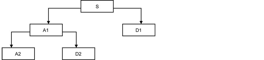
Figure 2. Multi-resolution analysis leading to the 2-levelde composition of a signal S.
2.2. Forecasting of Low-Frequency Signal Layers
The low frequency data which is gain by wavelet decomposing change slowly, so that it can be regard as steady time array, and forecasted with ARMA model. The low frequency data which was received using the wavelet decomposing methods were changing slowly, so it was regarded as a steady time array, so ARMA model was adopted to predict the share price.
The ARMA model is usually applied to auto correlated time series data. This model is a great tool for understanding and predicting the future value of a specified time series. ARMA is based on two parts: autoregressive (AR) part and moving average (MA) part [13] . Also, this model is usually referred as ARMA (p, q). In which p and q are the order of AR and MA respectively. A time series {Lt; t = 0, ±1, ±2, ∙∙∙} is ARMA (p, q) if it is stationary and:
 (6)
(6)
The parameters p and q are called the autoregressive and the moving average orders, respectively. {et; t = 0, ±1, ±2, ∙∙∙} is a Gaussian white noise sequence.  and
and  are constants.
The Akaike information criterion (AIC) can also be applied to decide the order of ARMA model. AIC is a measure of the goodness of fitting an estimated model. It is based on the concept of entropy. Entropy is a measure of the information lost when a mathematical model is used to describe the actual data. AIC is a powerful tool for model selection. The model with the lowest AIC has the best performance. The AIC is defined by the following equation:
 (7)
(7)
where  is the estimated value of
  which is the variance of the ARMA.
2.3. Forecasting of Intermediate-Frequency Signal Layers
The intermediate frequency data which is gain by wavelet decomposing is non-steady, so that it can be regard as steady time array, and forecasted with Kalman filter. The intermediate frequency data that received by using wavelet decomposing method was non-steady, so adopting the Kalman Filter was used to predict future forecasting.
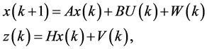
Kalman Filter is introduced and developed by Kalman [14] , and it is known as the most prominent adaptive method of state variables and data assimilation theme. The KF is the minimum variance estimation in linear systems within the realm of stochastic dynamic mode. The method consecutively estimates the state variables of models after measuring them. The detailed derivation of Kalman filtering can be found in [15] . In this section, only the necessary equation for the development of the basic recursive discrete Kalman filter will be addressed. Given the discrete state equations:
 (8)
(8)
where x(k) is system state vector, A and B are state transition matrix, z(k) is measurement vector, H is output matrix, W(k) is system error and V(k) is measurement error.
The recursive equations of Kalman filter are as following
 , (9)
, (9)
 , (10)
 , (11)
 , (12)
 . (13)
2.4. Forecasting of High-Frequency Signal Layers
The high-frequency data that was received by using wavelet decomposing methods was changing more violent with obvious randomness and non-linear characters, thus adopting the BP nerve network was used to predict future forecasts. In general, artificial neural networks (ANNs) possess attributes of learning, generalizing, parallel processing and error endurance. These attributes make the ANNs powerful in solving complex problems. Our study employs a BP neural network which is widely used in business situations.
A back-propagation network consists of at least three layers of units: an input layer, intermediate hidden layer, and an output layer (see Figure 3). Typically, units are connected in a feed-forward manner with input units completely connected to units in the hidden layer and hidden units completely connected to units in the output layer. When a B-P network runs and is cycled, an input pattern is propagated forward to the output units through the intervening input-to-hidden and hidden-to-output weights. Learning starts within a training phase and each input pattern in a training set is applied to the input units and then propagated forward. As the forward processing arrives at the
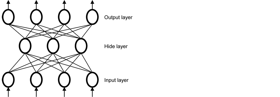
Figure 3. Back-propagation neural network.
output layer, the forward pattern is then compared with the correct (or observed) output pattern to calculate an error signal. The error signal for each such target output pattern is then back-propagated from the output layer to the input layer in order to appropriately amend or tune the weights in each layer of the network. After a B-P network has learned the correct classification for a set of inputs, it can be tested on a second set of inputs to see how well it classifies untrained patterns. Thus, an important consideration in applying B-P learning is how well the network generalizes. The detailed algorithm can be found elsewhere [16] and is, therefore, omitted in the text.
3. Application and Results
The data for our experiments are Shandong gold group closing prices, collected on the Shanghai Stock Exchange (SSE) market. The total number of values for the
There are two criteria for the selection of the mother wavelet. Firstly, the shape and the mathematical expression of the wavelet must be selected correctly so that the physical interpretation of the wavelet coefficients is easy. Secondly, the chosen wavelet must allow a fast computation of the required wavelet coefficients. In this paper, the discrete approximation of Meyer wavelet (D-Meyer) is hence selected as it is a fast algorithm which also supports discreet transformation [17] . The results in different scales are shown in Figure 5.
Figure 5 illustrates the three-level decomposition using D-Meyer. We can see from Figure 5(a), Figure 5(b) that the detailed scale mainly contains the trend component, Figure 5(c), Figure 5(d) represent most of the weekly periodic components and stochastic components. Figure 5(e), Figure 5(f) represent most of the strongly periodic components and stochastic components. So, A5 and D5 are low-frequency layers, D4 and D3 are intermediate-frequency layers, D2 and D1 high-frequency layers. Time series forecasting can be produced by forecasting on low-frequency, intermediate- frequency and high-frequency signal layers separately.
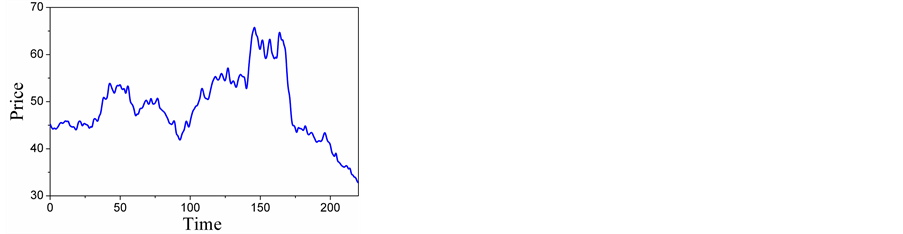
Figure 4. The original data.
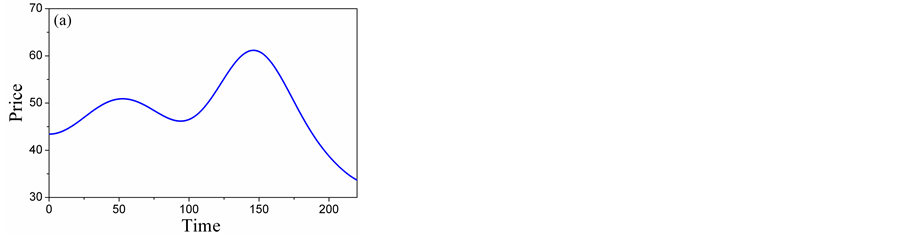
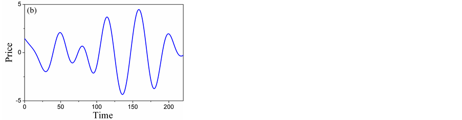
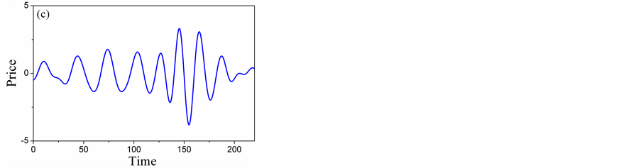
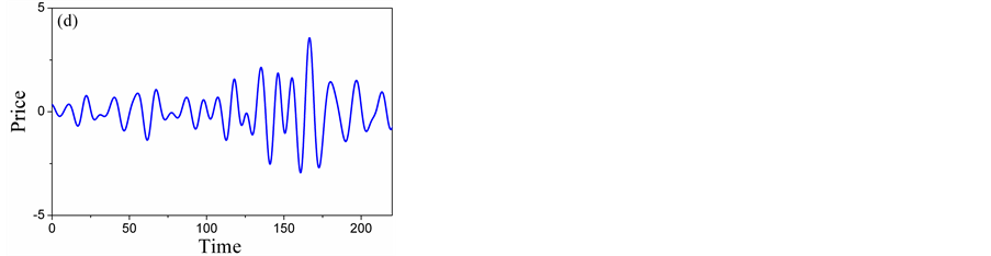
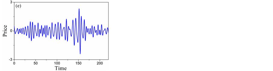
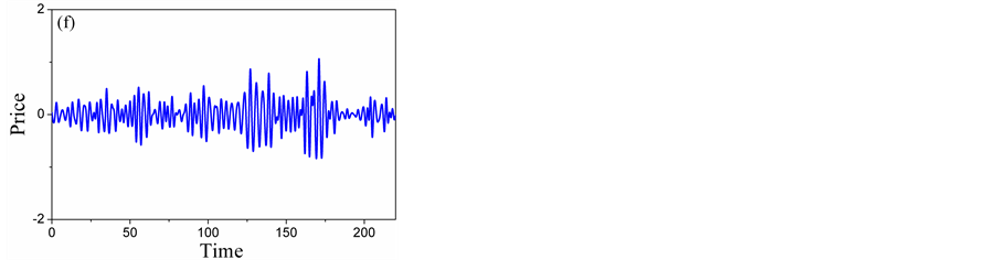
Figure 5. Five-level wavelet decomposition: (a) Detail of A5; (B) Detail of D5; (c) Detail of D4; (d) Detail of D3; (e) Detail of D2; (f) Detail of D1.
The ARMAS are employed to forecast low-frequency layers, and the forecasting results of A5 and D5 are shown in Figure 6. The Kalman Filters are employed to forecast low-frequency layers, and the forecasting results of D4 and D3 are shown in Figure 7. The BP neural networks are employed to forecast low-frequency layers, and the forecasting results of D2 and D1 are shown in Figure 8. The total forecasting results is shown in Figure 9. From the Figure 6 and Figure 9 it shows that, adopting multi-scale
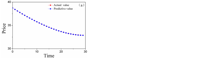
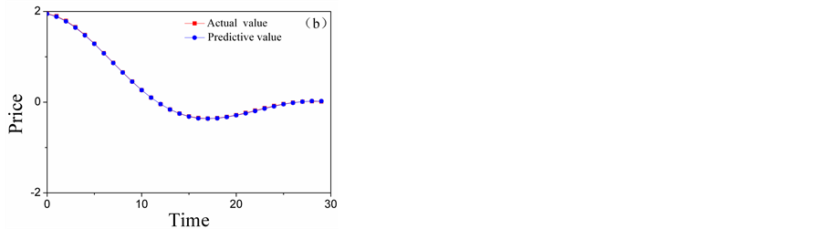
Figure 6. The comparison chart of the actual value and the forecasting results of high-frequency layers: (a) the comparison chart of A5; (b) the comparison chart of D5.
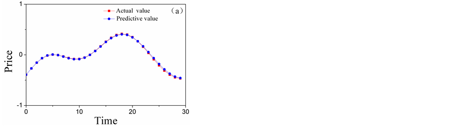
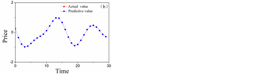
Figure 7. The comparison chart of the actual value and the forecasting results of high-frequency layers: (a) the comparison chart of D4; (b) the comparison chart of D3.
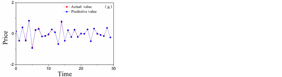
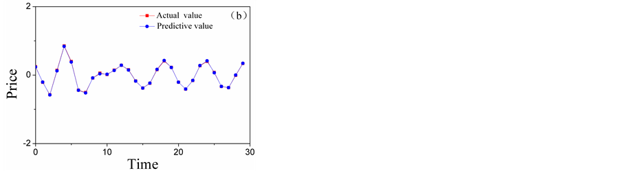
Figure 8. The comparison chart of the actual value and the forecasting results of high-frequency layers: (a) the comparison chart of D2; (b) the comparison chart of D1.
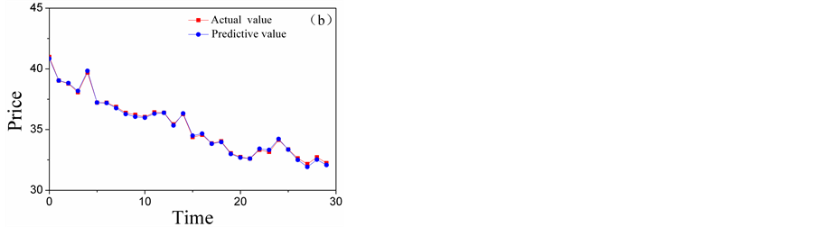
Figure 9. The comparison chart of the actual value and the forecasting results.
forecasting system the predicting results matching the reality data exactly. Therefore, multi-scale forecasting system was very effective.
4. Conclusion
The stock market data are highly random and non-stationary, and thus contain much noise. The lack of a good forecasting model motivates us to find an improved method of making forecasts called a hybrid forecasting system based on multiple scales. In this method, the original data are decomposed into multiple layers by the wavelet transform. And the multiple layers were divided into low-frequency, intermediate-frequency and high-frequency signal layers. Then autoregressive moving average (ARMA) models are employed for predicting the future value of low-frequency layers; Kalman filters are designed to predicting the future value of intermediate-frequency layers; and Back Propagation (BP) neural network models are established by the high-frequency signal of each layer for predicting the future value. Real data are used to illustrate the application of the hybrid forecasting system based on multiple scales, and the result of simulation experiments is excellent.
Cite this paper
Li, Y.Q., Li, X.B. and Wang, H.F. (2016) Based on Multiple Scales Forecasting Stock Price with a Hybrid Forecasting System. American Journal of In- dustrial and Business Management, 6, 1102- 1112. http://dx.doi.org/10.4236/ajibm.2016.611103
References
- 1. Armano, G., Marchesi, M. and Murru, A. (2005) A Hybrid Genetic-Neural Architecture for Stock Indexes Forecasting. Information Sciences, 170, 3-33.
https://doi.org/10.1016/j.ins.2003.03.023 - 2. Shumway, R.H. and Stoffer, D.S. (2014) Time Series Analysis and Its Applications. Springer-Verlag Inc., New York, 57.
- 3. Franses, P.H. and Ghijsels, H. (1999) Additive Outliers GARCH and Forecasting Volatility. International Journal of Forecasting, 15, 1-9.
https://doi.org/10.1016/S0169-2070(98)00053-3 - 4. Sarantis, N. (2001) Nonlinearities, Cyclical Behavior and Predictability in Stock Markets: International Evidence. International Journal of Forecating, 17, 459-482.
https://doi.org/10.1016/S0169-2070(01)00093-0 - 5. Konar, A. (2005) Computational Intelligence: Principles, Techniques. Springer, Berlin.
https://doi.org/10.1007/b138935 - 6. Khashei, M., Bijaria, M. and Ardali, G.A. (2009) Improvement of Auto-Regressive Integrated Moving Average Models Using Fuzzy Logic and Artificial Neural Networks (ANNs). Neurocomputing, 72, 956-967.
https://doi.org/10.1016/j.neucom.2008.04.017 - 7. Hansen, J.V. and Nelson, R.D. (2002) Data Mining of Time Series Using Stacked Generalizes. Neurocomputing, 43, 173-184.
https://doi.org/10.1016/S0925-2312(00)00364-7 - 8. Ture, M. and Kurt, I. (2006) Comparison of Four Different Time Series Methods to Forecast Hepatitis A Virus Infection. Expert Systems with Applications, 31, 41-46.
https://doi.org/10.1016/j.eswa.2005.09.002 - 9. Thawornwong, S. and Enke, D. (2004) The Adaptive Selection of Financial and Economic Variables for Use with Artificial Neural Networks. Neurocomputing, 56, 205-232.
https://doi.org/10.1016/j.neucom.2003.05.001 - 10. Peters, E.E. (1996) Fractal Market Analysis: Applying Chaos Theory to Investment and Economics. John Wiley & Sons, New York.
- 11. Gencay, R., Selcuk, F. and Whitcher, B. (2001) Wavelets and Other Filtering Methods in Finance and Economics. Academic Press, New York.
- 12. Burrus, C.S., Gopinath, R.A. and Guo, H. (1998) Introduction to Wavelets and Wavelet Transforms: A Primer. Prentice Hall, New Jersey.
- 13. Bruggemann, R. (2004) Model Reduction Methods for Vector Autoregressive Processes. Springer-Verlag, Berlin Heidelberg.
https://doi.org/10.1007/978-3-642-17029-4 - 14. Kalman, R.E. (1960) A New Approach to Linear Filtering and Prediction Problems. Journal of Basic Engineering, 82, 35-45.
https://doi.org/10.1115/1.3662552 - 15. Brown, R.G. (1983) Introduction to Random Signal Analysis and Kalman Filtering. Wiley, New York.
- 16. Haykin, S. (1999) Neural Networks: A Comprehensive Foundation. Prentice-Hall, New Jersey.
- 17. Enke, D. and Thawornwong, S. (2005) The Use of Data Mining and Neural Networks for Forecasting Stock Market Returns. Expert Systems with Applications, 29, 927-940.
https://doi.org/10.1016/j.eswa.2005.06.024