Open Journal of Civil Engineering
Vol.2 No.1(2012), Article ID:17821,7 pages DOI:10.4236/ojce.2012.21007
Urban Growth Modelling Using Determinism and Stochasticity in a Touristic Village in Western Greece
Laboratory of Soils and Agricultural Chemistry, Agricultural University of Athens Botanikos, Athens, Greece
Email: trdimitrios@gmail.com
Received December 5, 2011; revised January 10, 2012; accepted January 21, 2012
Keywords: Urban Growth Modelling; Determinism; Stochasticiy; Pogonia; Artificial Neural Network; Chaos Theory
ABSTRACT
Urban development has acquired an important magnitude in touristic places in Greece. Many villages, especially in seaside areas have adapted to touristic requirements by the necessary infrastructures and activities. Pogonia, located in Vonitsa Etoloakarnanias, is a village which has welcomed the opportunity of touristic development. As a result, the house settlements increased 57.5% during the last 8 years. Urban growth modelling using Artificial Neural Networks (ANNs) was applied in order to simulate the urban development in Pogonia village using two methods: determinism and stochasticity. The variables used for deterministic simulation were: distances to roads, urban areas and coastline, slope and elevation. It was found that urban development can be better described using the network of distances between all urban settlements (stochastic approach) rather than using determinism. This can be explained by the importance of the neighbourhood relationships and the interaction between urban settlements, occurred within the interconnected network of the self-organized urban system.
1. Introduction
Although urban areas cover a small percentage of the earth surface (2% - 3%), urbanization has increased during the last 200 years [1]. In 1800 only 2% of world population lived in urban areas, while in 1900 this ratio increased to 12% and in 2008 reached over 50%. As the urbanization grows, it is estimated that this percentage will approach to 75% by 2030 [2]. During the last decades it has been recognized that urban growth has produced many socioeconomic and environmental issues. Therefore, a large amount of urban growth models has appeared in order to study urban land use dynamics and simulate urban growth. The urban growth models have been developed based on two major analytical issues of spatial analysis: spatial autocorrelation and spatial heterogeneity. Spatial autocorrelation refers to the spatial variability of a driving force, according to the first law of Geography, in which near things are more similar than distant things. Spatial heterogeneity in an urban environment refers to the irregular distribution of urban settlements and therefore, urbanization produces spatial patterns.
Several approaches have been made in order to simulate urban growth. Some information will be given in the most usual urban growth models: 1) Spatial Statistics modeling; 2) Cellular Automata modelling; 3) Decision Trees modelling; 4) Artificial Neural Networks and 5) Fractal modeling.
Spatial statistics have been widely used in urban growth models [3-5]. The dependent variable can be estimated by independent variables using linear or multiple regression and logistic regression. In logistic regression, the dependent variable is dichotomous, which predicts the presence or absence of a characteristic. In case of spatial autocorrelation, an autocovariate term, which captures the spatial variability of the response variable, is added into regression equation [6]. The second important characteristic of urban growth is spatial heterogeneity [7]. Local models instead of a global model must be applied in areas with different patterns of urban growth [8,9].
Numerous models have been developed based on cellular automata for simulating urban growth since the last decades [10]. CA is discrete dynamics systems, represented by a grid of cells, where the state of each cell depends on the cell and its neighbours of its previous state, according to some transition rules. Many applications have used CA for urban growth modelling [11-14]. Some limitations of CA in urban simulation involve the spatial dimension, where global transition rules are not suitable for modeling cellular space. Moreover, the regularity of neighbourhoods is inappropriate, because neighbourhoods should be described my different shapes and sizes.
Decision trees automatically use some predefined rules in order to divide each variable. The smaller classes (nodes) produced correspond to a leaf of the decision tree and are associated with the branch produced by the upper-level nodes [15]. Although the large tree produced by the initial step of decision tree construction fits to the training set, it usually cannot predict new data with satisfactory accuracy. Pruning process is the necessary step, where smaller trees are produced with no noisy data and lower complexity [16,17]. There are two types of decision trees: 1) classification trees and 2) regression trees. In classification trees, the predicted variable takes only two values, while in the regression trees the predicted variable varies within the values of the dependent variable [16]. Spatial autocorrelation is a limitation in decision tree modeling [18,19]. This could be overcome using a proper sampling method, with large sampling distance [20]. Spatial heterogeneity is also another limitation in decision trees. [9] used an expert-based selection of local models, applied in different parts of the study area. This method performed better than applying a global model.
An Artificial Neural Network (ANN) is a system composed by single elements, called neurons. The output neurons are computed using an internal transfer function of the input neurons. The input neurons are related together with different weights. The ANN learns from the experience, using the input and output information through an iterative way of learning (e.g. back-propagation algorithm). ANNs are popular urban growth models. They have the advantage of no dependence on input data relationships. Therefore, they are free of assumptions about spatial autocorrelation and multi-collinearity. [21] produced the Land Transformation Model (LTM), where the land use changes were predicted using ANNs, considering social-economic and environmental factors. ART-MAP, another urban growth model, was produced by [22] using past information of land use and socio-economic data. ANNs have been also used in CA urban growth models for simulation and calibration [23,24]. ANN-based cellular automata models have been also applied for urban land use changes [25,26].
The nature is fractal itself, where the determinism and stochasticity co-exist within the self-organized natural system. In this system, the order and chaos are two phenomena which are alternated. Most urban growth models are deterministic, where the urban growth is predicted from the influence of some variables. The theory of chaos combines deterministic and stochastic approaches, applying non-linear dynamic oscillations of the urban characteristics. Therefore, future urban growth can be predicted by using self-similarity from urban characteristics. This approach can better simulate urban growth dynamics, once cities are fractals [27]. Cities are complex systems with characteristics of self-organisation, self-similarity and nonlinear relationships between urban settlements [12]. As it is explained above, the common philosophy of the urban growth models is the determinism, in which everything that happens depends on some variables; nothing else could happen. However, how easy is to include all the variables which influence the urban growth? If we included all the variables, would the urban growth be accurately predictable? Unfortunately neither it is easy to include all variables, nor will the prediction be accurate in case of including all variables. This can be explained as follows. Firstly, it is beyond human perceptive ability to find all the variables and secondly, there is the factor of randomness which plays an important role in a selforganized urban system. This gap is treated by chaos theory, where determinism and stochasticity can exist together.
In this research paper, the importance of the neighbourhood interactions between urban settlements is examined. These interactions represent the interconnected relationships in the urban self-organized urban network. It can be considered that this approach is a stochastic method because it does not take into account any independent variable which may influence urban growth, but it considers the self-similarity of distances between urban settlements. Therefore, the objective of this paper is to examine the determinism and stochasticity of the urbanisation by considering 1) independent variables which influence the urban growth (determinism) and 2) distances between urban settlements within the urban network (stochasticity) and 3) a combination of the two methods.
2. Study Area, Data Sources and Model Development
2.1. Study Area
The study area is located in the village of Pogonia, in Vonitsa Etoloakarnanias. It has a panoramic view in the gulf of Paleros, containing beaches all across the coast, and therefore, attracting many tourists. The Pogonia village is specified by Xmin: 224,994 m, Xmax: 226,221 m and Ymin: 4,297,944 m, Ymax: 4,299,157 m (Greek Grid), as Figure 1 presents. The urban settlements were extracted by digitizing orthophotographs and remote sensing imagery acquired by Google Earth and Hellenic Cadastre. Moreover, some more field work was taken place in order to complete and test the urban settlements. Therefore, two urban land use maps were produced for the years 2003 and 2011 respectively. From 142 urban settlements in 2003, covering an area of 18,379 m2, 50 more urban settlements were built since then, covering an area of 28,956 m2. The total urban growth is 57.5%, which is very important taking into account the time period of 8 years (2003 to 2011). Urban planners and decision makers in the municipality of Aktio-Vonitsas, where Pogonia village belongs, should try to keep the sustainability of environment, respecting the local people activities and traditions as well as the hospitality of the tourism.


Figure 1. Pogonia village (study area).
2.2. Response and Independent Variables
A grid of 50 m cellsize was produced, in which each cell was represented by a point. A total of 329 points were extracted from the whole study area and the model development was based on this point set. The response and the independent variables were calculated in these 329 points. The response variable is the urban development. It takes value 1 if non-urban areas of 2003 are converted to urban in 2011 and 0 if they remain non-urban. The urban areas of 2003 are excluded from the model development, because they are considered unconverted areas. The independent variables are: distance to roads (DistRoads), distance to urban areas (DistUrban) of 2003, distance to coastline (DistCoastline), elevation and slope. The Euclidean distance was used to calculate the distance variables. The cellsize used for the raster representation of these variables was 10 m. Statistical analysis of the study area showed that all the above variables contribute with high importance in urban growth modeling in Pogonia village. In order to better represent the importanceweight of each independent variable influencing urban growth, fuzzy sets were produced in each of them. The fuzzy values of the variables were used in model development.
In addition to the above independent variables, a network of interconnected distances was produced in order to evaluate the neighbourhood interaction between urban settlements. More specifically, the Euclidean distances from each of the 142 existed urban settlements in 2003 to the 329 points of the study area were calculated. Therefore, 142 variables with distances from each urban area were produced. This network of distances (DistNetwork) explains the non-linear relationships within the urban selforganized system.
2.3. Model Development
The model development was based in two principal components of chaos theory: determinism and stochasticity. Determinism takes into account the independent variables which influence urban growth, while stochasticity tries to model the non-linear interconnected relationships between urban settlements within the self-organized urban system. Except from examining determinism and stochasticity separately, a combination of them was also achieved.
More specifically, for stochasticity, 142 variables with distances between each house settlement in 2003 from 329 points of study area (DistNetwork) were considered in ANN-1 model. These 142 variables were standardized using maximum value. Therefore, they take values ranging from 0 to 1.
For determinism the fuzzy values of the following five independent variables: DistRoads, DistUrban, DistCoastline, Elevation and Slope were used as input neurons in the ANN-2 model. Fuzzy set theory is a generalization of Boolean logic, where there is no sharp boundaries between objects (variable values) which belongs to the set and those which do not. A membership function is applied into the variables, where each value takes a membership grade within 0 and 1 indicating the degree of its membership into the set. The value 1 indicates complete membership, while the value 0 non membership [28].
Moreover, a combination of these two approaches was produced using the ANN-3 model where the 142 standardized distance variables (DistNetwork) and the five fuzzy independent variables were included as input neurons. The output neuron in all ANN models was the dichotomous variable of urban changes from 2003 to 2011 (0: non urban to non urban and 1: non urban to urban).
The ANN models were applied to the point set of 329 locations. The initial dataset was divided to training set (60%), testing set (20%) and validation set (20%). For each ANN model 30 simulations were taken place, in which the best neural network (best validation accuracy) was finally selected. In each simulation 50 epochs (iterations) were achieved. Moreover, concerning the architecture of the ANN models, two hidden layers were used. Random nodes ranging from 8 to 16 and 1 to 6 were contained in each hidden layer respectively.
The design scheme of the model development is graphically presented in Figure 2. The application of the ANN models was achieved using appropriate code in Matlab environment.
3. Results and Discussion
The urban change is a dynamic phenomenon which is affected by many socioeconomic and biophysical factors. For examining the determinism, in each of the five independent variables: DistRoads, DistUrban, DistCoastline, Elevation and Slope, a corresponding fuzzy set was created by applying the SI model on the data of the year 2003. The membership function designed was based on expert knowledge and experience of the area and the statistical analysis of the data. Therefore, the independent variables favour urban growth as presented in Figure 3, where the fuzzy membership functions are drawn.
Distance to roads: Distances from roads less than 50 m positively influence urban growth. Therefore, they are assigned membership grade equal to 1 in the fuzzy set DistRoads. Distances greater than 50 m negatively influence urban growth, because the human factor is not intense in these areas. The crossover point of the membership function is at distance 90 m from roads. The width of the curve is 40 m.
Distance to urban areas: Close to urban areas, urban growth is increased. In distances less than 20 m the membership grade is equal to 1 in the fuzzy set DistUrban, while in distances greater than 20 m it varies from 0 to 1, taking the value 0.5 at distance equal to 50 m (crossover point). The width of the curve is 30 m.

Figure 2. Design scheme of urban growth modelling.
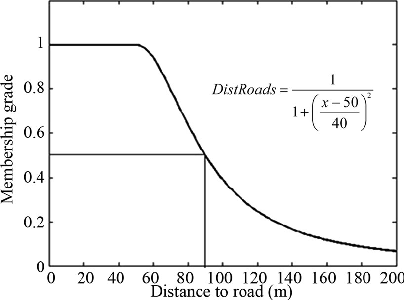
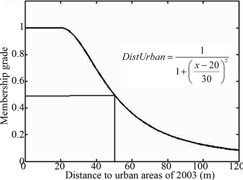
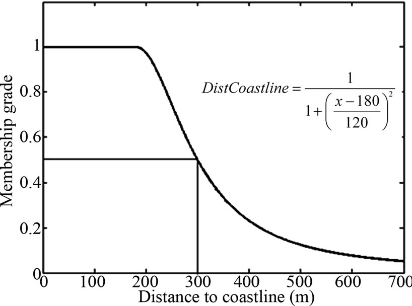
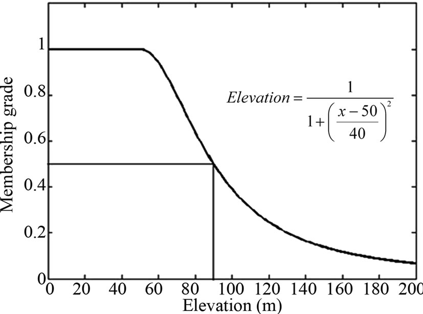

Figure 3. Fuzzy membership function of the independent variables of the urban growth in Pogonia village.
Distance to coastline: Areas near coastline favour urban growth. Therefore, in distances less than 180 m the membership grade takes the value of 1 in the fuzzy set DistCoastline. The fuzzy function gives membership grade equal to 0.5 (crossover point) to distance of 300 m. The width of the curve is 170 m.
Elevation: In low elevation the urban growth is increased. Elevation less than 50 m the membership grade is equal to 1. The membership function gives membership grade 0.5 at 90 m elevation. The width of the curve is 40 m.
Slope: Areas with slope less than 20% favour urban growth. Thus, these slopes take membership grade 1 in the fuzzy set Slope. Slopes greater than 20% take membership grades according to the membership function, where at 30% slope the membership grade is 0.5 (crossover point). The width of the SI curve is 10%.
The accuracy was calculated using the percentage of the correctly classified. Moreover, the Kappa statistic was also estimated in order to remove the cases, which were correctly classified by chance. The accuracy results of the three ANN models are presented in Table 1.
As the Table 1 shows, the model which produced the best results was the ANN-1, while the ANN-2 was the least important model. Therefore, considering only the 5 independent variables or examining the urban growth with deterministic approach, the results are not encouraged. The best results were produced using the distances between urban settlements only. This means that the stochasticity plays an important role in urban growth, because urban dynamics are sufficiently described by the interconnected relationships between urban settlements. Moreover, using all variables (ANN-3) where determinism meets stochasticity (ANN-3 variables: variables of ANN-1 plus those of ANN-2) the accuracy increased, but without achieving the best results. This gives the opportunity to remark the importance of stochasticity, which takes into account the self-similarity between connections of urban settlements as shown in Figure 4.
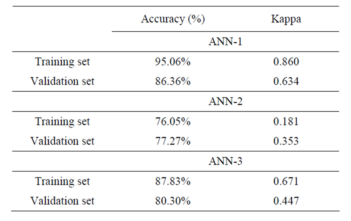
Table 1. Accuracy results of the ANN-1, ANN-2 and ANN-3 models.

Figure 4. Self similarity in the interconnected network of urban settlements 2003.
The lines between point 1 and the urban areas of 2003 as well as the dashed lines between point 2 and the same urban areas of 2003 (1, 2: two points of 329 total) are self-similar (Figure 4). The only difference is the scale which changes from point 1 to point 2. This self-similarity is one of the principles of chaos theory, which allows the examination of behaviour of dynamic systems. In this study area, the best results were produced considering the self-similarity of urban connections and their simulation in ANN-1 model.
4. Conclusions
In this research paper, determinism and stochasticity were considered in order to simulate urban growth in Pogonia village, western Greece. Determinism was evaluated using five independent variables (DistRoads, DistUrban, DistCoastline, Elevation and Slope), which influence urban growth, while stochasticity was approached using distances between urban settlements, which indicates the interconnected relationships within the urban self-organised system.
The results showed that stochasticity produces better performance than determinism or combination of the two of them. This is very important outcome because it is usually difficult to consider all the independent variables which actually influence urban growth. Although applying deterministic approaches into real world phenomena is an important part of scientific research, stochasticity was proved to play a protagonistic role in this research. Therefore, according to chaos theory, which acts as a bridge between determinism and stochasticity, it can be generally argued that stochasticity must co-exist with determinism because they both scientifically and philosophically explain the urban growth complexity more appropriately.
REFERENCES
- L. Poelmans and V. A. Rompaey, “Complexity and Performance of Urban Expansion Models,” Computers, Environment and Urban Systems, Vol. 34, No. 1, 2010, pp. 17-27. doi:10.1016/j.compenvurbsys.2009.06.001
- UNFPA, 2007. http://www.unfpa.org/public/
- X. Li and A. G. Yeh, “Analyzing Spatial Restructuring of Land Use Patterns in a Fast Growing Region Using Remote Sensing and GIS,” Landscape and Urban Planning, Vol. 69, No. 4, 2004, pp. 335-354. doi:10.1016/j.landurbplan.2003.10.033
- M. Herold, H. Couclelis and K. C. Clarke, “The Role of Spatial Metrics in the Analysis and Modeling of Urban Land Use Change,” Computers, Environment and Urban Systems, Vol. 29, No. 4, 2005, pp. 369-399. doi:10.1016/j.compenvurbsys.2003.12.001
- K. McGarigal, S. Tagil and S. Cushman, “Surface Metrics: An Alternative to Patch Metrics for the Quantification of Landscape Structure,” Landscape Ecology, Vol. 24, No. 3, 2009, pp. 433-450. doi:10.1007/s10980-009-9327-y
- M. Deng, “A Spatially Autocorrelated Weights of Evidence Model,” Natural Resources Research, Vol. 19, No. 1, 2010, pp. 33-44. doi:10.1007/s11053-009-9107-z
- J. Liu and W. W. Taylor, “Integrating Landscape Ecology into Natural Resource Management,” Cambridge University Press, Cambridge, 2002.
- A. Paez and D. Scott, “Spatial Statistics for Urban Analysis: A Review of Techniques with Examples,” GeoJournal, Vol. 61, No. 1, 2005, pp. 53-67. doi:10.1007/s10708-005-0877-5
- D. Triantakonstantis, G. Mountrakis and J. Wang, “A Spatially Heterogeneous Expert Based (SHEB) Urban Growth Model Using Model Regionalization,” Journal of Geographic Information System,Vol. 3, No. 3, 2011, pp. 195-210. doi:10.4236/jgis.2011.33016
- I. Santé, A. M. García, D. Miranda and R. Crecente, “Cellular Automata Models for the Simulation of RealWorld Urban Processes: A Review and Analysis,” Landscape and Urban Planning, Vol. 96, No. 2, 2010, pp. 108- 122. doi:10.1016/j.landurbplan.2010.03.001
- R. White, G. Engelen and I. Uljee, “The Use of Constrained Cellular Automata for High-Resolution Modelling of Urban Land-Use Dynamics,” Environment and Planning B: Planning and Design, Vol. 24, No. 3, 1997, pp. 323-343. doi:10.1068/b240323
- J. I. Barredo, M. Kasanko, N. McCormick and C. Lavalle, “Modelling Dynamic Spatial Processes: Simulation of Urban Future Scenarios through Cellular Automata,” Landscape and Urban Planning, Vol. 64, No. 3, 2003, pp. 145-160. doi:10.1016/S0169-2046(02)00218-9
- A. D. Syphard, K. C. Clarke and J. Franklin, “Using a Cellular Automaton Model to Forecast the Effects of Urban Growth on Habitat Pattern in Southern California,” Ecological Complexity, Vol. 2, No. 2, 2005, pp. 185-203. doi:10.1016/j.ecocom.2004.11.003
- J. Vliet, R. White and S. Dragicevic, “Modeling Urban Growth Using a Variable Grid Cellular Automaton,” Computers, Environment and Urban Systems, Vol. 33, No. 1, 2009, pp. 35-43. doi:10.1016/j.compenvurbsys.2008.06.006
- J. R. Quinlan, “Probabilistic Decision Tress,” In: K. Yves and R. Michalski, Eds., Machine Learning: An Artificial Intelligence Approach, Volume III, San Mateo, Morgan Kaufmann, 1983, pp. 140-152.
- K. M. Osei-Bryson, “Post-Pruning in Decision Tree Induction Using Multiple Performance Measures,” Computers & Operations Research, Vol. 34, No. 11, 2007, pp. 3331-3345. doi:10.1016/j.cor.2005.12.009
- W. Cheng, K. Wang and X. Zhang, “Implementation of a COM-Based Decision-Tree Model with VBA in Arc GIS,” Expert Systems with Applications, Vol. 37, No. 1, 2010, pp. 12-17. doi:10.1016/j.eswa.2009.01.006
- J. A. F. Diniz-Filho, L. M. Bini and B. A. Hawkins, “Spatial Autocorrelation and Red Herrings in Geographical Ecology,” Global Ecology and Biogeography, Vol. 12, No. 1, 2003, pp. 53-64. doi:10.1046/j.1466-822X.2003.00322.x
- B. Lees, “The Spatial Analysis of Spectral Data: Extracting the Neglected Data,” Applied GIS, Vol. 2, No. 2, 2006, pp. 14.1-14.13.
- F. E. Nelson, K. M. Hinkel, N. I. Shiklomanov, G. R. Mueller, L. L. Miller and D. A. Walker, “Active-Layer Thickness in North Central Alaska: Systematic Sampling, Scale, and Spatial Autocorrelation,” Journal of Geophysical Research, Vol. 103, No. D22, 1998, pp. 28963- 28973. doi:10.1029/98JD00534
- B. C. Pijanowski, D. G. Brown, B. A. Shellito and G. A. Manik, “Using Neural Networks and Gis to Forecast Land Use Changes: A Land Transformation Model,” Computers, Environment and Urban Systems, Vol. 26, No. 6, 2002, pp. 553-575. doi:10.1016/S0198-9715(01)00015-1
- W. Liu and K. C. Seto, “Using the ART-MMAP Neural Network to Model and Predict Urban Growth: A Spatiotemporal Data Mining Approach,” Environment and Planning B: Planning and Design, Vol. 35 No. 2, 2008, pp. 296-317. doi:10.1068/b3312
- C. M. Almeida, J. M. Gleriani, E. F. Castejon and B. S. Soares-Filho, “Using Neural Networks and Cellular Automata for Modelling Intra-Urban Land-Use Dynamics,” International Journal of Geographical Information Science, Vol. 22, No. 9, 2008, pp. 943-963. doi:10.1080/13658810701731168
- Y. Mahajan and P. Venkatachalam, “Neural Network Based Cellular Automata Model for Dynamic Spatial Modeling in GIS,” Springer, Berlin/Heidelberg, 2009, pp. 341-352.
- B. Pijanowski, S. Pithadia, B. Shellito and A. Alexandridis, “Calibrating a Neural Network-Based Urban Change Model for Two Metropolitan Areas of the Upper Midwest of the United States,” International Journal of Geographical Information Science, Vol. 19, No. 2, 2005, pp. 197- 215. doi:10.1080/13658810410001713416
- Q. Guan, L. Wang and K. C. Clarke, “An Artificial-Neural-Network-Based, Constrained CA Model for Simulating Urban Growth,” Cartography and Geographic Information Science, Vol. 32, No. 4, 2005, pp. 369-380. doi:10.1559/152304005775194746
- M. Batty and P. A. Longley, “Fractal Cities: A Geometry of Form and Function,” Academic Press, London, 1994.
- L. A. Zadeh, “Fuzzy Sets,” Information and Control, Vol. 8, 1965, pp. 338-353. doi:10.1016/S0019-9958(65)90241-X