Received 19 August 2014; revised 10 September 2014; accepted 18 September 2014

ABSTRACT

Studying the dynamical behaviors of the liquid spike formed by Rayleigh-Taylor instability is important to understand the mechanisms of liquid atomization process. In this paper, based on the information on the velocity and pressure fields obtained by the coupled-level-set and volume-of- fluid (CLSVOF) method, we describe how a freed spike can be formed from a liquid layer under falling at a large Atwood number. At the initial stage when the surface deformation is small, the amplitude of the surface deformation increases exponentially. Nonlinear effect becomes dominant when the amplitude of the surface deformation is comparable with the surface wavelength (~0.1λ). The maximum pressure point, which results from the impinging flow at the spike base, is essential to generate a liquid spike. The spike region above the maximum pressure point is dynamically free from the bulk liquid layer below that point. As the descending of the maximum pressure point, the liquid elements enter the freed region and elongate the liquid spike to a finger-like shape.

Keywords:

Fluid Mechanics, Multi-Phase Flow, Rayleigh-Taylor Instability, Spike Formation

1. Introduction

When an external acceleration directs from a light fluid to a heavy one, instability takes place on the interface, which is usually called Rayleigh-Taylor (RT) instability. One of the most familiar phenomena associated with the RT instability in our daily life is the water falling from the ceiling. The RT instability also plays an important role in the formation of supernova [1] [2] , ignition in the inertial confinement fusion (ICF) [3] [4] , and liquid atomization [5] [6] .

The RT instability was first described mathematically by Rayleigh [7] . Later, Taylor [8] conducted a linear analysis on the RT instability in the absence of the surface tension and viscosity. He derived that the amplitude of the initial disturbance grows exponentially over time. Lewis [9] then observed the RT instability for various experimental conditions. He found that the instability development agreed well with the linear theory proposed by Taylor [8] until the amplitude was comparable with the wavelength l. When the surface amplitude becomes large, the development must be treated as a nonlinear process. The light fluid penetrates the heavy fluid as a bubble and the heavy fluid penetrates the light fluid as a spike. Several models have been proposed to describe the nonlinear dynamics. Layzer [10] obtained an approximate analytic solution for the instability of a fluid-va- cuum interface in a gravitational field. In such case of limited Atwood number, where r_H is the density for the heavy fluid and r_L for the light fluid, he find that the bubble velocity is a constant value eventually, which is proportional to (gl)^1/2, where g is the gravitational acceleration. Goncharov [11] generalized the result of Layzer [10] to arbitrary Atwood numbers for both two-dimensional (2D) and three-di- mensional (3D) geometries. The bubble velocity predicted by these models has been validated by various experimental studies [12] - [15] .

In experiments, it is difficult to control the initial disturbance, while it is easy to be conducted in numerical simulations. Furthermore, the numerical simulation can provide us information on the detailed flow-field data, which are difficult to measure in experiments. Thus, as the development of computer capacity and numerical schemes, more numerical investigations have been conducted to study the RT instability [16] - [19] .

Most of the previous studies focused on the bubble behavior, especially on the constant velocity of the rising bubble. However, for applications of RT instability to some fields, e.g., the liquid atomization, the spike behaviors are of greater interest. Ramaprabhu et al. [18] have pointed out that the spike behaves similar to the bubble for a_t far smaller than unity and approaches a free-fall for a_t being close to unity. In the liquid atomization field, in which a_t approaches unity, we have to reveal the mechanism of how the spike develops freely from the bulk liquid based on the detailed information on pressure and velocity. To our knowledge, few investigations have studied this. Although Baker et al. [20] have conducted a numerical study on the effects of liquid depth on the bubble speed and the spike acceleration, the detailed physics associated with that how a liquid spike is formed are not discussed. Therefore, we conduct the present numerical simulation. As the first step to study the problem in 3D case, which requires large calculation time, we first pay attention to 2D case in this study.

2. Problem Statement and Numerical Setups

2.1. Physical Model

In this 2D study, as shown in Figure 1, we consider an inviscid liquid layer lying on a falling plate. The liquid density is r_l, and the gas density is r_g. For numerical stability, the density ratio is set to be r_l/r_g = 100. The corresponding Atwood number is a_t = 0.98, which approaches unity. The surface tension coefficient on the liquid-gas interface is s. The plate falls with acceleration (A + g). In the reference frame attached to the plate, the governing equations to be solved are Euler equations

(1)

where u is the velocity vector, r is the density, p is the pressure, e_y is the unit vector along y-direction, and F_s represents the surface tension force according to the continuum surface force (CSF) method [21] . According to the dispersion relation including viscosity obtained by Piriz et al. [22] , the viscous damping effects are negligible if k³n² = A for a large Atwood number (a_t → 1), where n is the liquid kinematic viscosity coefficient. Thus, the calculation results based on the inviscid assumption are valid for the condition k³n²/A = 1.

As shown in Figure 1, the horizontal dimension of the calculation domain was one wavelength, L_x= λ = 2p/k. The depth of the liquid layer was h₀ = l. Baker et al. [20] has pointed out that the liquid depth effects are significant only when the depth becomes smaller than ~0.5λ. In the present study, though the liquid surface trough moves downwards as time elapses, the smallest liquid depth is still around 0.5l at the end of the calculation (see Figure 3), which indicates that the liquid depth effects were negligible throughout the present calculations. The vertical direction of the gas phase was 1.5λ, with the purpose to offer enough room for the growth of liquid spike. Thus, the entire vertical dimension of the calculation domain was L_y = 2.5λ.

Equation (1) was non-dimensionalized with the characteristic time t_s = (l/A)^1/2, the characteristic length l_s = l, the characteristic velocity u_s = (lA)^1/2, and the characteristic pressure p_s = r_l Al. In the following, we denoted the dimensionless quantities with a superscript^*. After non-dimensionalization, a dimensionless parameter A^* was derived as

. (2)

2.2. Boundary and Initial Conditions

The boundary and initial conditions were imposed into the calculation domain as shown in Figure 1. Since we only consider a normal mode RT instability, the cyclic boundary conditions were imposed on the left and right edges. The bottom edge was a slip wall due to the negligibility of viscosity in this study. The top was a free edge. We initiated the disturbance with a sinusoidal vertical velocity distribution on the liquid surface. = 0.001 was set in this study.

2.3. Numerical Setups

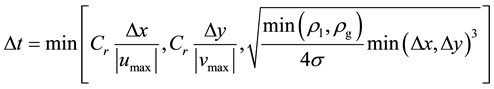
A uniform and staggered mesh was used to discretize the governing equations. The governing equations were solved based on the “marker-and-cell (MAC)” method [23] . A tentative velocity field excluding the pressure term was first computed. A second order upwind scheme was used to discretize the convective term. Then, a pressure Poisson equation with the divergence of the tentative velocity as the source term will be solved to determine the pressure field at the new time step. Finally, the velocity field at the new time step is updated by the determined pressure field. The liquid-gas interface was captured by the coupled-level-set and volume-of-fluid (CLSVOF) method [24] [25] . The LS function f, which is the normal distance from the interface, is naturally a continuous function and thus can evaluate the interface curvature correctly, but it loses the mass-conserving in the re-initialization process. The VOF function F, which is the volume fraction in each calculation grid, is naturally mass-conserving, but its step-like property introduces more errors in the curvature evaluation. The CLSVOF method takes advantages of both methods. The details of the numerical methods to be used can be found in Ref. [25] . The grid size was set to be Δ = Δx = Dy = l/64, which is the finest one used by Ramaprabhu and Dimonte [26] . The time step at each calculation instant is restricted by two considerations, i.e., materials (e.g., free surface) and capillary waves cannot move more than the size of one cell in one time step, which can be expressed as

(3)

where C_r is the Courant number, which is set to be 0.25 in this study.

3. Results and Discussions

In this study, we conducted a series of calculations of the dimensionless parameters A^* ranging from 2.4p³ to 8.8p³, with an interval of 0.8p³. The similar spike formation structure was observed for these cases. Thus, we discuss the major dynamics associated with the spike formation due to RT instability based on the prototype case of A^*= 4.48p³. A typical corresponding physical condition is r_l = 1000 kg/m³, r_g = 10 kg/m³, λ = 5 cm, s = 0.073 N/m, A = 4.35 m/s².

3.1. Surface Evolution

Figure 2 shows the temporal evolution of the shape of liquid (dark region) surface. At the beginning, the surface is in a flat shape and a disturbance is introduced on the surface. Then the surface shape deforms continuously with time. According to the linear theory [7] [22] , the amplitude of the surface deformation d grows exponentially as

, (4)

which is depicted as the solid line in Figure 3. Until about t^* = 2.4, the surface is in a sinusoidal shape and the magnitude of the surface deformation is small. Therefore, as shown in Figure 3, the evolutions of the absolute value of surface elevation at the spike tip (x^* = 0.25) and the trough bottom (x^* = 0.75) agree well with the linear prediction. After t^* = 2.4, the amplitude of the surface deformation is no longer a small value compared with the wavelength (d ^* > 0.1). The nonlinearity becomes dominant and the calculation results depart from the linear prediction. It is noticeable that the trough bottom descends with a steady velocity after t^* = 2.4. This is a typical nonlinear phenomenon associated with the RT instability, which has been studied extensively before [10] [11] . Based on an approximate potential flow model, Goncharov [11] derived an expression of the constant descending velocity as V = [A/(3k)]^1/2 for the large Atwood number in 2D configuration. Using the characteristic velocity u_s = (lA)^1/2 in this study, the dimensionless descending velocity is V^* = 0.23, which is close to our calculation results (V^* = 0.225 as shown in Figure 3). Since the Atwood number approaches unity in this study, the Kelvin-

Helmholtz instability [15] , occurring on the surface of the upward moving spike when the densities of two fluids are comparable, is not observed.

3.2. Dynamical Structures

To understand the process of spike formation due to RT instability, we should study the liquid spike structure in detail. Figure 4 shows the vertical pressure distributions along the spike centerline (Figure 4(a)) and the trough centerline (Figure 4(b)). According to the different dynamical characteristics, we divided the liquid spike into three regions, which are discussed as below.

Region A In the Region A near the plate, as shown in Figure 4, the pressure distributions are almost identical along the spike centerline and the trough centerline. Because the liquid flow is limited around the surface, the magnitude of the velocity away from the surface is small. Thus, the linear theory, which predicts the vertical distribution of vertical velocity v(y) µ sinh(ky), is valid in Region A. This means that there is a region in which the expression lg[v^*(y^*)] µ 2p lge・y^* in dimensionless form should be valid. In Figure 5, we showed that the vertical distribution of the vertical velocity along the spike centerline at t^* = 3.6 and t^* = 4.0, when the surface deformation is large. It can be seen that the numerical results of the velocity distribution in Region A are consistent with the linear theory, which indicates that for a thick liquid layer, the dynamics in the region away from the surface can be described by the linear theory and this region is not important for the spike formation from the liquid surface.

Region B The formation of the spike is greatly dependent on the dynamics in Region B. The most important dynamic occurring in the spike base region (Region B) is the formation of the maximum pressure point after t^* = 3.2, as shown in Figure 4(a). Figure 6 demonstrates the flow field and the pressure contours near the spike base. The liquid flow from the neighboring troughs collides at the spike base. This impinging flow increases the pressure at the spike base, which inhibits the liquid elements entering spike region and deviates the calculation results from the linear prediction as shown in Figure 3. When the magnitude of the liquid velocity increases large enough, a local maximum pressure point is formed at the spike base. The formation of the maximum pressure point, where the vertical pressure gradient dp^*/dy^* is zero, results in the liquid above the maximum pressure point (Region C) dynamically free from the bulk liquid layer below the maximum pressure point. As shown in Figure 4(a), the maximum pressure point descends with time. The liquid elements entering the spike region elongate the spike and result in a finger-like shape. An interesting phenomenon is shown in Figure 7, which shows the temporal evolution of the dimensionless distance x^* between the maximum pressure point and the trough bottom after the maximum pressure point forms. x^* almost keeps at a same value around 0.35, which indicates that the maximum pressure point descends with the trough bottom as a whole.

Region C As shown in Figure 4(a), the pressure in the liquid region above the maximum pressure point is nearly uniform along the spike centerline except in the tip region, where the capillary pressure is important. For a finger-like liquid spike, as shown in Figure 2, the surface (except the bulbous tip) is in a shape of nearly

straight-line, the curvature of which is small. Thus, the liquid pressure in the spike region is close to the gas pressure around, which is almost uniform due to the large density ratio considered in this study. The vertical momentum equation of a liquid element in Region C can be expressed as

(5)

where y*(t*) is the vertical position of the liquid element. Then, we obtained the solution of Equation (5)

, (6)

where and are the vertical velocity and the vertical position at. Figure 8 shows the temporal evolution of the vertical position of a liquid element which locates at and holds at. It clearly shows that the vertical position of the liquid element in Region C is well described by Equation (6), which is consistent with the free-fall behavior of the liquid spike concluded by He et al. [27] for large Atwood number.

4. Conclusions

By using the CLSVOF method, we numerically studied the mechanisms of the spike formation due to RT instability for a large Atwood number. The following conclusions were reached.

1. At the initial stage, the amplitude of the surface deformation increases exponentially, which can be described by linear theory.

2. For a thick liquid layer, there is a region away from the surface, in which the linear theory is valid even when the surface deformation is large.

3. The local maximum pressure point, which is formed by the impinging flow at the spike base, is essential to the formation of a freed spike.

4. The element in the liquid spike region above the maximum pressure point is dynamically freed from the bulk liquid layer below the maximum pressure point, which approaches a free-fall.

Cite this paper

YikaiLi,AkiraUmemura, (2014) Mechanism of the Large Surface Deformation Caused by Rayleigh-Taylor Instability at Large Atwood Number. Journal of Applied Mathematics and Physics,02,971-979. doi: 10.4236/jamp.2014.210110

References

NOTES

^*Corresponding author.

References

- 1. Arnett, W.D., Bahcall, J.N., Kirshner, R.P. and Woosley, S.E. (1989) Supernova 1987A. Annual Review of Astronomy and Astrophysics, 27, 629-700. http://dx.doi.org/10.1146/annurev.aa.27.090189.003213
- 2. Norman, M., Smarr, L., Smith, M. and Wilson, J. (1981) Hydrodynamic Formation of Twin-Exhaust Jets. Astrophysical Journal, 247, 52-58. http://dx.doi.org/10.1086/159009
- 3. Evans, R., Bennett, A. and Pert, G. (1982) Rayleigh-Taylor Instabilities in Laser-Accelerated Targets. Physical Review Letters, 49, 1639-1642. http://dx.doi.org/10.1103/PhysRevLett.49.1639
- 4. Lindl, J.D., McCrory, R.L. and Campbell, E.M. (1992) Progress toward Ignition and Burn Propagation in Inertial Confinement Fusion. Physics Today, 45, 32-40. http://dx.doi.org/10.1063/1.881318
- 5. Beale, J.C. and Reitz, R.D. (1999) Modeling Spray Atomization with the Kelvin-Helmholtz /Rayleigh-Taylor Hybrid Model. Atomization Sprays, 9, 623-650. http://dx.doi.org/10.1615/AtomizSpr.v9.i6.40
- 6. Kong, S., Senecal, P. and Reitz, R. (1999) Developments in Spray Modeling in Diesel and Direct-Injection Gasoline Engines. Oil & Gas Science and Technology, 54, 197-204.
http://dx.doi.org/10.2516/ogst:1999015 - 7. Rayleigh, L. (1883) Investigation of the Character of the Equilibrium of an Incompressible Heavy Fluid of Variable Density. Proceedings of the London Mathematical Society, 14, 170-177.
- 8. Taylor, G.I. (1950) The Instability of Liquid Surfaces When Accelerated in a Direction Perpendicular to Their Planes. I. Proceedings of the Royal Society A, 201, 192-196. http://dx.doi.org/10.1098/rspa.1950.0052
- 9. Lewis, D. (1950) The Instability of Liquid Surfaces When Accelerated in a Direction Perpendicular to Their Planes. II. Proceedings of the Royal Society A, 202, 81-96.
- 10. Layzer, D. (1955) On the Instability of Superposed Fluids in a Gravitational Field. Astrophysical Journal, 122, 1-12.
http://dx.doi.org/10.1086/146048 - 11. Goncharov, V. (2002) Analytical Model of Nonlinear, Single-Mode, Classical Rayleigh-Taylor Instability at Arbitrary Atwood Numbers. Physical Review Letters, 88, Article ID: 134502.
http://dx.doi.org/10.1103/PhysRevLett.88.134502 - 12. Andrews, M.J. and Dalziel, S.B. (2010) Small Atwood Number Rayleigh-Taylor Experiments. Philosophical Transactions of the Royal Society A: Mathematical Physical and Engineering Sciences, 368, 1663-1679.
- 13. Dimonte, G., Ramaprabhu, P., Youngs, D., Andrews, M. and Rosner, R. (2005) Recent Advances in the Turbulent Rayleigh-Taylor Instability. Physics of Plasmas, 12, Article ID: 056301.
http://dx.doi.org/10.1063/1.1871952 - 14. Ramaprabhu, P. and Andrews, M. (2004) Experimental Investigation of Rayleigh-Taylor Mixing at Small Atwood Numbers. Journal of Fluid Mechanics, 502, 233-271.
http://dx.doi.org/10.1017/S0022112003007419 - 15. Waddell, J., Niederhaus, C. and Jacobs, J. (2001) Experimental Study of Rayleigh-Taylor Instability: Low Atwood Number Liquid Systems with Single-Mode Initial Perturbations. Physics of Fluids (1994-Present), 13, 1263-1273.
http://dx.doi.org/10.1063/1.1359762 - 16. Baker, G.R., Meiron, D.I. and Orszag, S.A. (1980) Vortex Simulations of the Rayleigh-Taylor Instability. Physics of Fluids (1958-1988), 23, 1485-1490. http://dx.doi.org/10.1063/1.863173
- 17. Ramaprabhu, P., Dimonte, G. and Andrews, M. (2005) A Numerical Study of the Influence of Initial Perturbations on the Turbulent Rayleigh-Taylor Instability. Journal of Fluid Mechanics, 536, 285-320.
http://dx.doi.org/10.1017/S002211200500488X - 18. Ramaprabhu, P., Dimonte, G., Woodward, P., Fryer, C., Rockefeller, G., Muthuraman, K., Lin, P. and Jayaraj, J. (2012) The Late-Time Dynamics of the Single-Mode Rayleigh-Taylor Instability. Physics of Fluids (1994-Present), 24, Article ID: 074107. http://dx.doi.org/10.1063/1.4733396
- 19. Youngs, D.L. (1984) Numerical Simulation of Turbulent Mixing by Rayleigh-Taylor Instability. Physica D: Nonlinear Phenomena, 12, 32-44. http://dx.doi.org/10.1016/0167-2789(84)90512-8
- 20. Baker, G., Verdon, C., McCrory, R. and Orszag, S. (1987) Rayleigh-Taylor Instability of Fluid Layers. Journal of Fluid Mechanics, 178, 161-175. http://dx.doi.org/10.1017/S0022112087001162
- 21. Brackbill, J., Kothe, D.B. and Zemach, C. (1992) A Continuum Method for Modeling Surface Tension. Journal of Computational Physics, 100, 335-354. http://dx.doi.org/10.1016/0021-9991(92)90240-Y
- 22. Piriz, A., Cortázar, O., Cela, J.L. and Tahir, N. (2006) The Rayleigh-Taylor Instability. American Journal of Physics, 74, 1095-1098. http://dx.doi.org/10.1119/1.2358158
- 23. Harlow, F.H. and Welch, J.E. (1965) Numerical Calculation of Time-Dependent Viscous Incompressible Flow of Fluid with Free Surface. Physics of Fluids (1958-1988), 8, 2182-2189.
http://dx.doi.org/10.1063/1.1761178 - 24. Sussman, M. and Puckett, E.G. (2000) A Coupled Level Set and Volume-of-Fluid Method for Computing 3D and Axisymmetric Incompressible Two-Phase Flows. Journal of Computational Physics, 162, 301-337.
http://dx.doi.org/10.1006/jcph.2000.6537 - 25. Van der Pijl, S., Segal, A., Vuik, C. and Wesseling, P. (2005) A Mass-Conserving Level-Set Method for Modelling of Multi-Phase Flows. International Journal for Numerical Methods in Fluids, 47, 339-361.
http://dx.doi.org/10.1002/fld.817 - 26. Ramaprabhu, P. and Dimonte, G. (2005) Single-Mode Dynamics of the Rayleigh-Taylor Instability at Any Density Ratio. Physical Review E, 71, Article ID: 036314. http://dx.doi.org/10.1103/PhysRevE.71.036314
- 27. He, X., Zhang, R., Chen, S. and Doolen, G.D. (1999) On the Three-Dimensional Rayleigh-Taylor Instability. Physics of Fluids (1994-Present), 11, 1143-1152.