Journal of Applied Mathematics and Physics
Vol.2 No.7(2014), Article
ID:46808,12
pages
DOI:10.4236/jamp.2014.27061
On the Existence and Uniqueness of Solutions for Nonlinear System Modeling Three-Dimensional Viscous Stratified Flows
Andrei Giniatoulline, Tovias Castro
Department of Mathematics, Los Andes University, Bogota, Colombia
Email: aginiato@uniandes.edu.co, te.castro37@uniandes.edu.co
Copyright © 2014 by authors and Scientific Research Publishing Inc.
This work is licensed under the Creative Commons Attribution International License (CC BY).
http://creativecommons.org/licenses/by/4.0/


Received 1 March 2014; revised 1 April 2014; accepted 8 April 2014
ABSTRACT
We establish the uniqueness and local existence of weak solutions for a system of partial differential equations which describes non-linear motions of viscous stratified fluid in a homogeneous gravity field. Due to the presence of the stratification equation for the density, the model and the problem are new and thus different from the classical Navier-Stokes equations.
Keywords:Partial Differential Equations, Sobolev Spaces, Fluid Dynamics, Stratified Fluid, Viscous Fluid

1. Introduction
The objective of this paper is to study the qualitative properties of the weak solutions of the system of partial differential equations which describes nonlinear motions of stratified three-dimensional viscous fluid in the gravity field, such as existence, uniqueness and smoothness. This model of three-dimensional stratified fluid corresponds to a stationary distribution of the initial density in a homogeneous gravitational field, which is of Boltzmann type and is exponentially decreasing with the growth of the altitude. The results may be applied in the mathematical fluid dynamics modelling real non-linear flows in the Atmosphere and the Ocean.
The additional unknown function (density), as well as the stratification equation itself, constitutes the novelty of the problem. To construct the solutions, we will use the Galerkin method.
We consider a bounded domain  with the boundary of the class
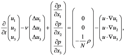
  piecewise, and the following system of fluid dynamics
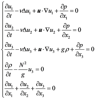 (1.1)
(1.1)
Here  is the space variable,
  is the velocity field,
  is the scalar field of the dynamic pressure and
  is the dynamic density. In this model, the stationary distribution of density is described by the function
 , where N is a positive constant. The gravitational constant g and the viscosity coefficient
  are also assumed as strictly positive.
For linear non-viscous case, Equations (1.1) are deduced, for example, in [1] -[3] . For linear viscous compressible fluid, system 1.1 is deduced, for example, in [4] . The linear system corresponding to 1.1, was studied from various points of view, and some results may be found in [5] -[10] .
There exists, of course, huge bibliography concerning Navier-Stokes system (see, for example, [11] -[14] ).
However, the non-linear system modelling stratified viscous flows have not been studied mathematically yet, and thus our research was motivated by the novelty of the presence of the term ![]() in the third equation of 1.1, and also by the presence of the fourth equation itself.
in the third equation of 1.1, and also by the presence of the fourth equation itself.
2. Construction and Existence of a Weak Solution
We denote  and observe that, without loss of generality we can consider
 . In this way, we write Equations (1.1) in the vector form:
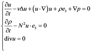 (1.2)
(1.2)
We associate system 1.2 with the initial conditions
 (1.3)
(1.3)
and the Dirichlet boundary conditions
 . (1.4)
Let ![]() be a functional space of smooth solenoidal functions with compact support in Ω. We denote as
be a functional space of smooth solenoidal functions with compact support in Ω. We denote as  the closure of
 ![]() in the norm
in the norm . We also denote as
  the space of solenoidal functions from
 ![]() which satisfy homogeneous Dirichlet condition.
which satisfy homogeneous Dirichlet condition.
Definition 1.
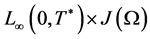
Let
 ,
, .
.
For any pair of vector functions  we denote
 .
.
We will call  a weak solution of 1.2-1.4, if the following integral identities hold
 (1.5)
(1.5)
 (1.6)
(1.6)
for every pair of functions  such that
![]() ,
, ![]() , and
, and 
We observe that the relations 1.5 - 1.6 are obtained in a natural way after multiplying by  the system 1.2, and integrating by parts over
 ![]() for x and over the interval
for x and over the interval  for t. After knowing the functions
 , the function
  can be easily found from 1.2.
Let  be a complete orthonormal system in
 . We observe that, without loss of generality, it can be chosen as a system of eigenfunctions of Stokes operator (see, for example, [11] [13] [15] ).
We construct the solutions of 1.2 as Galerkin approximations
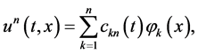 (1.7)
(1.7)
where ![]() are unknown coefficients and
are unknown coefficients and  are obtained as solutions of Cauchy problem
![]() (1.8)
(1.8)
Our primary aim is to determine the existence of  and the resulting properties of the approximations
 .
.
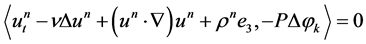
If we consider 1.5 for  and
and![]() then, the arbitrary election of
then, the arbitrary election of  will imply the relations
 (1.9)
(1.9)
We transform now the system 1.9 into an autonomous system of differential equations of the first order with respect to the variables , where the vector field is
 . If we denote
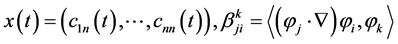 , then it can be easily seen that the system 1.9 is equivalent to
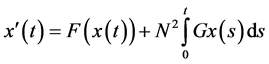 , (1.10)
where
 ,
,
 ,
,
 .
.
After differentiating 1.10, we obtain
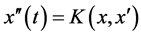 , (1.11)
where 
We introduce the notation  and thus rewrite 1.11 as
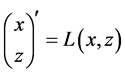 . (1.12)
Since  is an infinitely differentiable vector field, then, from the theory of ordinary differential equations, we conclude that 1.12 admits a maximal solution in the interval
 .
.
Now, we shall deduce some estimates to prove that  is independent on
 .
.
Lemma 1.
The solutions ![]() of the approximate system 1.9 are defined uniquely by 1.7.
of the approximate system 1.9 are defined uniquely by 1.7.
Additionally, the following estimates are valid. For all ![]() there exists
there exists 
such that 1) 
2)  for all
3) 
4)  for all
5)  for all
6)  for all
where the positive constants a, b, M and  depend only on the initial data 1.3, the parameter of the system N and the domain
![]() .
.
Remark.
The values of the constants a, b, M and  are given below in 1.22, 1.28 and 1.29.
Proof.
For ![]() we introduce the following auxiliary real-valued function
we introduce the following auxiliary real-valued function .
.
We observe that
 . (1.13)
After multiplying each equation of 1.9 by  and summing them with respect to
 , we obtain
 .
.
In this way, choosing , we have that
 . (1.14)
Therefore, 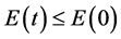 for all t, and thus
 . (1.15)
In particular, we have . Thus the statement “a)” of the Lemma is proved.
From 1.14 we obtain that
 (1.16)
which will prove the statement “b)”. Indeed,

Now, differentiating 1.9, we obtain .
.
We multiply the last relations by  and sum them with respect to k:
 .
.
Therefore, keeping in mind that , we have
 . (1.17)
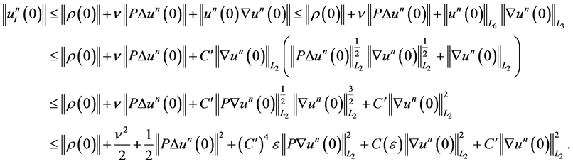
We would like to estimate the right-hand terms in 1.17. Evidently, from 1.15 we obtain
 (1.18)
We will need the following estimate:
 (1.19)
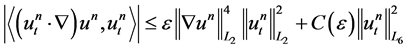
On the other hand, from the generalized Hölder inequality and the interpolation inequality
 , we can estimate the term
 (1.20)
From the Young inequality with “ε” for ,
,  ,
,  ,
, we obtain
 (1.21)
Now, using 1.19 and the inclusion Sobolev inequality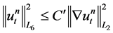 , we have

If we choose  such that
 , then the last estimate, together with 1.17 and 1.18, implies
 (1.22)
Evidently, from 1.22 we have
 , (1.23)
from which, after integrating with respect to t, it follows that
 . (1.24)
Now, to obtain a uniform upper estimate with respect to n for , we only need to prove such estimate for
 . We remind that the system
 , being formed by eigenfunctions of Stokes operator is orthonor mal in
 , and also in
  with the scalar product
 , as well as in
 ![]() with the scalar product
with the scalar product , where P is an orthogonal projection of
  onto
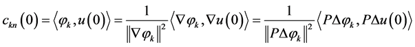
onto . From 1.9 we have
 .
.
Proceeding analogously to 1.17-1.21 and also using Lemma 1 from [11], we obtain
If we choose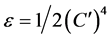 , then we finally have
 (1.25)
Now, from the Bessel inequality and the properties
 , (1.26)
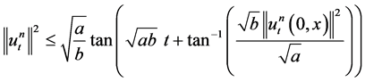
we can express 1.25 as
 (1.27)
In this way, using 1.27 and the evident inequality , we can estimate 1.24 as
 (1.28)
where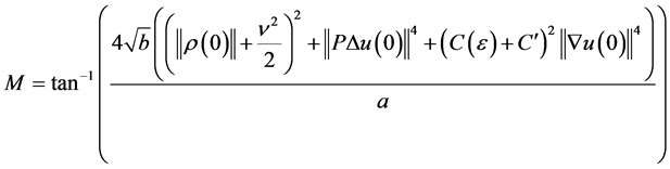 .
.
Taking , we assure that
  and thus we obtain the result that for all
![]() there exists
there exists  such that
 , (1.29)
which proves the statement “c)” of the Lemma. It is easy to see that the statement “d)” is a direct consequence of 1.19 and 1.29. The statement “e)” of the Lemma is obtained immediately if we integrate both sides of 1.29 with respect to t. It remains to prove the statement “f)”. For that, we use 1.15 and 1.16 and therefore obtain
 which concludes the proof of the Lemma.
We would like to obtain now more estimates for the approximate solutions ![]() with an intention to show that their limit, which is an obvious candidate for a solution of 1.2 - 1.4, would preserve certain regularity properties of
with an intention to show that their limit, which is an obvious candidate for a solution of 1.2 - 1.4, would preserve certain regularity properties of 
Lemma 2.
For all ![]() and for all
and for all  there exists a constant
 ![]() which does not depend on
which does not depend on , such that the following estimate is valid:
Proof.
We continue using the notation of P as an orthogonal projection of  onto
onto . Let
. Let ![]() be eigenvalues corresponding to the eigenfunctions
be eigenvalues corresponding to the eigenfunctions  of the Stokes operator. We multiply 1.9 by
  and sum up the resulting equations with respect to
 . In this way, we have
 . (1.31)
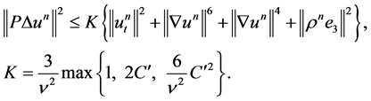
We would like to estimate the following term in 1.31:
 . (1.32)
By using Cauchy and Hölder inequality, together with the inequality , we obtain
 . (1.33)
Now we use Sobolev inclusion inequality and Lemma 1 from [11], which allows us to estimate 1.33 as
 (1.34)
We take , consider the inequality
 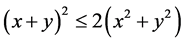 and use the property
 .
.
Proceeding in this way, we obtain
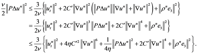
Now, if we take , we will finally have
 (1.35)
The term  on the right side of 1.35 can be estimated by 1.29. The terms
 , can be estimated analogously, we use the statement “d)” of Lemma 1 and the inequality
 where we consider p = 2 and p = 3. Now, taking into account the properties
 (1.36)
 (1.37)
we can proceed estimating the integral of 1.35 as follows:
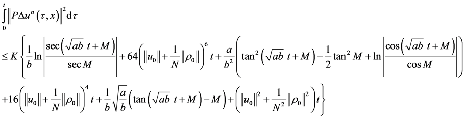
(1.38)
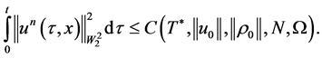
We note that the estimate 1.38 is valid for . From 1.28 - 1.29 we have that the value
  is chosen in such a way that the right side of 1.38 is positive. Finally, we use the result from [15] where there is shown that in the functional space
![]() , the norms
, the norms  and
and  are equivalent, which concludes the proof.
Theorem 1.
Let  be a bounded domain with the boundary of the class
 , and let
![]() ,
,
 .
.
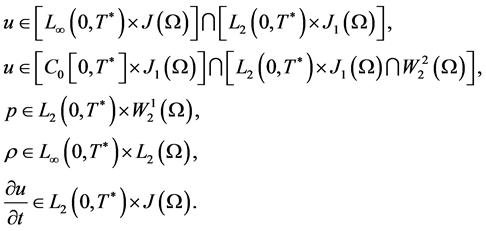
Then, there exists an interval  and there exist the functions
  which satisfy the system 1.2 and the conditions 1.3 - 1.4 in sense of 1.5 - 1.6, such that
Proof.
From Lemma 1 and Lemma 2 we have that there exist a function u and a subsequence of  (which, for brevity, we will denote also as
 ), such that
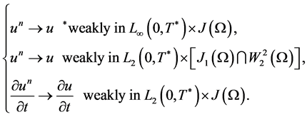 (1.39)
We note that the inclusion  is compact and continuous, and that
  is bounded in
 from Lemma 1. On the other hand, from the statement “c)” of Lemma 1 we have that for
 and
and , the following estimate holds:
 (1.40)
In this way, from 1.39, 1.40 and Lemma 24.5 [12], it follows that  belongs to a compact set in
 . Therefore, the subsequence in 1.39 can be chosen in such a way that
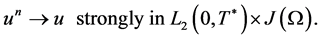 (1.41)
It is easy to see that u satisfies the regularity properties of the Theorem. Indeed, since
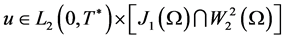 and
and  then, from Theorem IV.5.11 [15] we obtain that
 . Using Sobolev inequality we have the estimate

Therefore, ; which, in turn, implies
 . Nowlet us show that u satisfies 1.5. Evidently,
  and
and  satisfy 1.5 for
 (1.42)
Since , then

Analogously, we have that  It remains to prove the limit
 (1.43)
To verify 1.43, we note first that
 (1.44)
We integrate by  the relation 1.44 and use the properties that
 ![]() is uniformly bounded in
is uniformly bounded in
 and that
  In this way, we obtain that 1.43 is valid.
Now, we pass to the limit for  in
in
 and thus obtain
 (1.45)
for the functions  from 1.42. Due to the density of the set 1.42, we have that 1.45 is valid for all the functions
  from Definition 1, which completes the proof.
2. Uniqueness of the Solutions
Theorem 2.
The weak solution in sense of Definition 1, is unique.
Proof.
Let us exchange ![]() by
by  and thus rewrite the system 1.2 in a more symmetrical way:
 (2.1)
(2.1)
 (2.2)
(2.2)
Let  and
and  be two solutions of 2.1 - 2.2 which satisfy the conditions 1.3 - 1.4 and also the conditions of Theorem 1. We denote
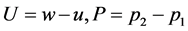 , and thus obtain
 (2.3)
(2.3)
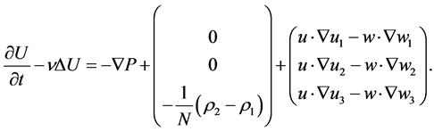
From 2.2 we have . We observe that we can express 2.3 as follows:
 (2.4)
(2.4)
We multiply 2.4 by U, integrate by parts in . In this way, we have
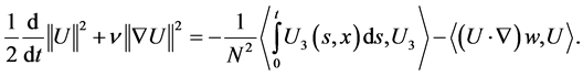 (2.5)
(2.5)
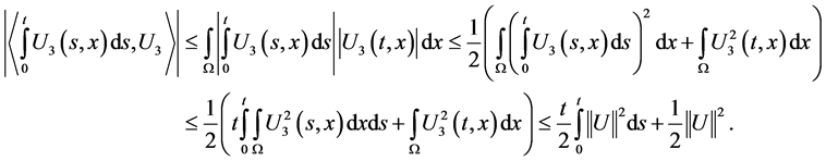
By using the generalized Hölder inequality and Young inequality, together with the inequity
 , we can estimate the last term in 2.5 as
 (2.6)
(2.6)
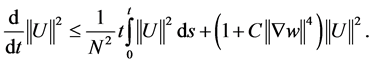
If we take , then we will have the estimate
 (2.7)
(2.7)
Now we would like to estimate the term . It is easy to see that
In this way, from 2.7 we obtain the estimate
 (2.8)
(2.8)
Now, let us consider the following initial value problem for the function :
:
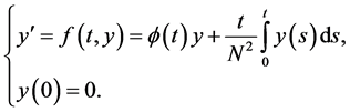 (2.9)
(2.9)
Evidently, for continuous  the unique solution of the problem 2.9 is
 .
.
By comparison principle, therefore, for every solution of the differential inequality

the property holds:  In this way, we conclude from 2.9 that
 , which implies that
 .
.
Using 2.2 we obtain also that , and thus the theorem is proved.
Acknowledgements
This research was partially supported by “Fondo de Investigaciones Facultad de Ciencias-Uniandes”.
References
- Cushman-Roisin, B. and Beckers, J. (2011) Introduction to Geophysical Fluid Dynamics. Academy Press, New York.
- Tritton, D. (1990) Physical Fluid Dynamics. Oxford UP, Oxford.
- Kundu, P. (1990) Fluid Mechanics. Academy Press, New York.
- Landau, L. and Lifschitz, E. (1959) Fluid Mechanics. Pergamon Press, New York.
- Makarenko, N., Maltseva, J. and Kazakov, A. (2009) Conjugate Flows and Amplitude Bounds for Internal Solitary Waves. Nonlinear Processes in Geophysics, 16, 169-178. http://dx.doi.org/10.5194/npg-16-169-2009
- Maurer, B., Bolster, D. and Linden, P. (2010) Intrusive Gravity Currents between Two Stably Stratified Fluids. Journal of Fluid Mechanics, 647, 53-69. http://dx.doi.org/10.1017/S0022112009993752
- Birman, V. and Meiburg, E. (2007) On Gravity Currents in Stratified Ambients. Physics of Fluids, 19, 602-612. http://dx.doi.org/10.1063/1.2756553
- Maslennikova, V. and Giniatoulline, A. (1992) On the Intrusion Problem in a Viscous Stratified Fluid for Three Space Variables. Mathematical Notes, 51, 374-379. http://dx.doi.org/10.1007/BF01250548
- Giniatoulline, A. and Zapata, O. (2007) On Some Qualitative Properties of Stratified Flows. Contemporary Mathematics, Series AMS, 434, 193-204.
- Giniatoulline, A. and Castro, T. (2012) On the Spectrum of Operators of Inner Waves in a Viscous Compressible Stratified Fluid. Journal of the Faculty of Science, University of Tokyo, 19, 313-323.
- Heywood, J. (1980) The Navier-Stokes Equations: On the Existence, Regularity and Decay of Solutions. Indiana University Mathematics Journal, 29, 639-681. http://dx.doi.org/10.1512/iumj.1980.29.29048
- Tartar, L. (2006) An Introduction to Navier-Stokes Equations and Oceanography. Springer, Berlin.
- Temam, R. (2000) Navier-Stokes Equations: Theory and Numerical Analysis. AMS Chelsea Publishing, New York.
- Sohr, H. (2012) The Navier-Stokes Equations: An Elementary Functional Analytic Approach. Birkhuser, Zurich.
- Boyer, F. (2005) Elements d’analyse pour l’etude de quelques modeles d’ecoulements de fluides visqueux incompressibles. Springer, Berlin.