Journal of Applied Mathematics and Physics
Vol.2 No.4(2014), Article ID:43973,7 pages DOI:10.4236/jamp.2014.24007
The Lagrangian Method for a Basic Bicycle
F. Talamucci
DIMAI, Dipartimento di Matematica e Informatica “Ulisse Dini”, Università degli Studi di Firenze, Firenze, Italy
Email: federico.talamucci@math.unifi.it
Copyright © 2014 by author and Scientific Research Publishing Inc.
This work is licensed under the Creative Commons Attribution International License (CC BY).
http://creativecommons.org/licenses/by/4.0/


Received 16 February 2014; revised 11 March 2014; accepted 18 March 2014
ABSTRACT
The ground plan in order to disentangle the hard problem of modelling the motion of a bicycle is to start from a very simple model and to outline the proper mathematical scheme: for this reason the first step we perform lies in a planar rigid body (simulating the bicylcle frame) pivoting on a horizontal segment whose extremities, subjected to nonslip conditions, oversimplify the wheels. Even in this former case, which is the topic of lots of papers in literature, we find it worthwhile to pay close attention to the formulation of the mathematical model and to focus on writing the proper equations of motion and on the possible existence of conserved quantities. In addition to the first case, being essentially an inverted pendulum on a skate, we discuss a second model, where rude handlebars are added and two rigid bodies are joined. The geometrical method of Appell is used to formulate the dynamics and to deal with the nonholonomic constraints in a correct way. At the same time the equations are explained in the context of the cardinal equations, whose use is habitual for this kind of problems. The paper aims to a threefold purpose: to formulate the mathematical scheme in the most suitable way (by means of the pseudovelocities), to achieve results about stability, to examine the legitimacy of certain assumptions and the compatibility of some conserved quantities claimed in part of the literature.
Keywords:Nonholomic Constraints; Lagrangian Equations; Pseudovelocities; Nonlinear Order Differential Equations; Stability

1. Introduction
1.1. The Equations of the Model
A very simple scheme can be formulated by assuming that the body is a planar rigid system  sketched by three points A, B and
![]() ; A and B, performing the two contact points of the wheels, belong to a horizontal plane and
; A and B, performing the two contact points of the wheels, belong to a horizontal plane and ![]() is the centre of mass of
is the centre of mass of . The rigid body can lean with respect to the vertical direction and bend with respect to a fixed horizontal direction. Let O be the projection of
 ![]() on
on  and take a fixed reference frame
 ,
,  being the upward vertical, and a body reference frame
  such that
 ![]()
is the angle ,
, ![]() is the angle
is the angle . The mutual disposal of the two frames is given by

and sketched in Figure 1.
Set : the geometrical restrictions
 ,
,  ,
,  lead us to consider the four lagrangian coordinates
 . Therefore
 . The angular velocity of the rigid body is
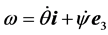 .
.
The Lagrangian function of the system writes
 (1)
(1)
where  and
and ,
,  and
and  are the moments of inertia with respect to the body reference frame
 , which is supposed to be principal.
The only kinetic constraint we are going to consider is , whose expression in the Lagrangian coordinates is
 (2)
(2)
The first kind Lagrangian equations of motion
 (3)
(3)
where 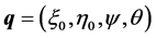 are the lagrangian coordinates and
 ![]() is the unknown multiplier, will be suitably handled if one defines the pseudovelocities (see [1] for the concepts and the method we are pursuing)
is the unknown multiplier, will be suitably handled if one defines the pseudovelocities (see [1] for the concepts and the method we are pursuing)
 (4)
(4)
We point out the following relationships involving U, V and the real velocities:
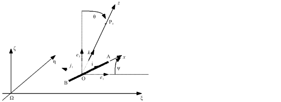
Figure 1. The geometrical model.
 (5)
(5)
where  and
and 
Together with the kinetic constraint, Equations (4) give the set of possible velocities in terms of :
:
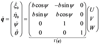 (6)
(6)
It is known (see [1] ) that linear kinetic constraints allow to refine the equations of motion (3) in a way similar to the holonomic case: as a matter of fact, the constraints identify a subspace in the tangent space of the lagrangian coordinates, giving the virtual displacement of the system. The geometrical method consists of projecting the equations according to  where
where  is defined in (6). Joining to the kinetic constraint (2) and the definition (4) we get, dividing by suitable constants,
 (7)
(7)
where
 (8)
(8)
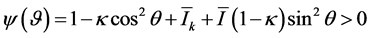
are dimensionless constants. Since the rigid body is practically plane and contained in the plane orthogonal to j, it is reasonable to assume ,
,  , so that
 (9)
(9)
From here on we adopt (9).
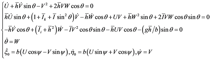
The seven ODEs (7) contain the seven unknown quantities . With respect to the first kind system (3) they have the advantage of no exhibiting multipliers and of reducing the kinetic variables of one unity.
It is not at all worthless to explain (7) in the context of the the cardinal equations of dynamics, seeing that many models in literature (some of them are [2] -[5] ) rest on such equations: the first three equations in (7) are respectively
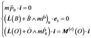
where L is the angular momentum and  the resultant momentum of the external forces. Actually, since no friction is present, the constraint
  in A is along
 , while the constraints in B can be modelled as a force
  along
along  plus a horizontal force
  perpendicular to
  (see Figure 2), acting the constraint (2):
 (10)
(10)
Hence no force exists along ![]() (first equation) and
(first equation) and  (second equation), along
  (and not
![]() , as stated in [6] ). Finally, third equation is simply due to the fact that the only external force with a non zero momentum along
, as stated in [6] ). Finally, third equation is simply due to the fact that the only external force with a non zero momentum along ![]() is the weight force.
is the weight force.
Notice that any of the three equations do not give rise to a conserved quantity: the only evident constant of
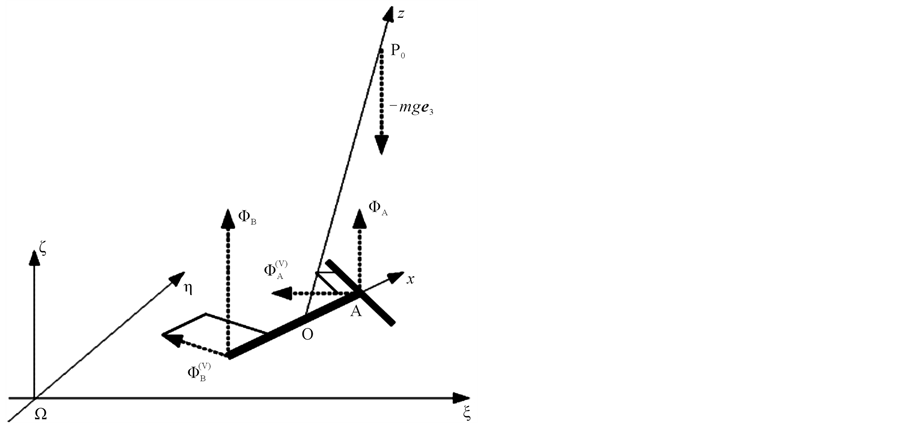
Figure 2. The system of forces.
motion is the total energy :
:
 (11)
(11)
Actually, even if the system is nonholonomic, the first integral  can be achieved starting from
 and performing the usual calculations as in the holonomic case, achieving at last
![]() .
.
In the same matter of integral invariants for the system, we find it not correct to claim, as in [7] , that the absence of ,
,  ,
, ![]() from
from ![]() entails three constant of motion, in order that four conserved quantities (including the total energy) can be obtained: as a matter of fact, the equations of the model are not
entails three constant of motion, in order that four conserved quantities (including the total energy) can be obtained: as a matter of fact, the equations of the model are not 
and cyclic variable does not mean conserved quantity. Besides that, even if ![]() is written in terms of
is written in terms of ![]() and
and![]() ,
, ![]() is not a cyclical coordinate, being implicitily in such variables. For this reason we question the validity of
is not a cyclical coordinate, being implicitily in such variables. For this reason we question the validity of  (Equation (14) in [7] ), which would imply an integral invariant.
With regards to the same subject, we emphasize that equation  (Equation (16) in [7] ), giving rise to the conservation of
 , is not correct in our advice, since U does not refer to a lagrangian coordinate.
1.2. The Mathematical Problem
We perform now a brief analysis of (7). It is evident that the first four equations in (7) form the sub-system
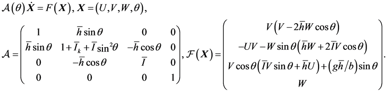 (12)
(12)
The last three equations in (7) give simply![]() ,
, ![]() ,
, ![]() once (12) has been solved.
once (12) has been solved.
Statement 1.1 System (7) admits locally one solution, for any set of data ,
,  ,
,  ,
,  ,
,  ,
,  ,
, .
.
Proof. The assigned data provide  and
and , by means of (6). Furthermore
 (13)
(13)
where we defined (see also (8) and (9))
 (14)
(14)
Therefore (12) can be solved in an appropriate time interval. Finally one obtains![]() ,
, ![]() e
e ![]() from the last three equations in (7) and the rest of the given data. □
from the last three equations in (7) and the rest of the given data. □
Remark 1.1 If in (7) we let , we are dealing with the simpler case of a bar on a horizontal plane with one point moving at each time along the direction of the bar: since
 ![]() equations reduce to
equations reduce to

The energy conservation  gives the orbits on the phase plane
 , namely each point of the
 ![]() -axis and the semi-ellipses
-axis and the semi-ellipses . Moreover
 ,
,  , that is
 ,
, .
.
Again for![]() , the special case
, the special case , that concerns with one typical instance in nonholonomic constraints (see for instance [1] ), cannot be recovered from the system of Remark 1.2, but it requires the definition of the pseudovelocity
 .
.
We are going now to investigate the stability of the system at![]() .
.
For what concerns with the initial data, we can certainly assume with no loss in generality ,
,  ,
,  , hence
 .
.
Let us first check whenever  is a solution of (7).
Statement 1.2  is solution of (7) if and only if U is constant and
![]() .
.
Proof. Set ![]() in (7), first three equations:
in (7), first three equations:

which entails![]() ,
, . We incidentally notice that if
  then U, V consistent with
 ![]() are those we discussed in Remark 1.3.
are those we discussed in Remark 1.3.
On the other hand, U constant and ![]() make us write (12), second and third equation, as
make us write (12), second and third equation, as
 (15)
(15)
(it is physically correct to assume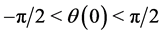 ), which implies
 . □
. □
Remark 1.2 The following statement also follows from the previous analysis: if the angle ![]() is constant (that is
is constant (that is  never changes direction), then U has to be constant and
  has to be zero.
Corollary 1.1 Assume ,
, ; then
  is solution of (7) if and only if
 .
.
Proof. If ![]() is solution, then
is solution, then ![]() must be zero at any time; on the other hand, the set of data
must be zero at any time; on the other hand, the set of data ,
,  ,
,  ,
,  give univocally the solution
 ,
,  ,
, . □
. □
Our aim points now to discuss the stability of . Thre physical problem requires
  (see (5)). Incidentally we notice that if
  is the solution of (7) starting from
 , then
  is the solution of the same equations corresponding to
 .
.
It may be helpful by the way to set ![]() in (7) in order to figure out the behaviour of the solution for short times:
in (7) in order to figure out the behaviour of the solution for short times:
 (16)
(16)
that is, assuming for istance ,
,  , U and W are initially increasing, V decreasing.
Let us now show the following Proposition 1.1 The equilibrium point  of (12) is unstable.
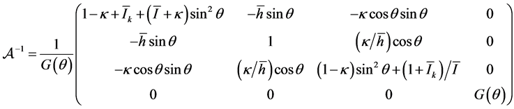
Proof. We set (12) in normal form: calling , where
  is computed in (13), it is easily found
so that  can be calculated (see (12) for
![]() ).
).
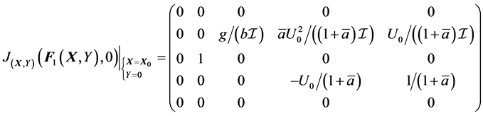
We now compute the Jacobian matrix of  at the equilibrium
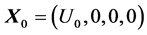 : calculations lead to
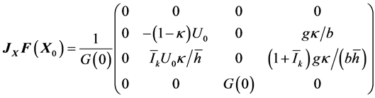
where . The eigenvalues
  are found by solving
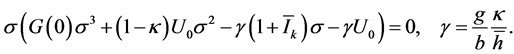 (17)
(17)
Since , the polynomial
  in brackets is such that
  and
and , so that there exists one real and positive eigenvalue
  and standard results in this sense (see e.g. [8] ) can be implemented. □
The linear approximation  entails
  and
and
 (18)
(18)
which give the equation for![]() :
:
 (19)
(19)
whose solution contains ,
, . As to
 , the linear approximation gives

which diverges the same.
An analytical investigation can be performed directly for system (7): choosing for istance, as it is natural,  ,
,  and
and , (16) shows that
 ![]() initially increases, so that P0 enters the quarter
initially increases, so that P0 enters the quarter . Furthermore, setting
![]() ,
,  one writes (7) as
with appropriate![]() ,
, ; on the other hand, using also

which is (11) with the appropriate G, one should acquire information about the maintenance of ![]() (
( does not change verse), of
 ![]() (the transverse velocity of O is opposite to the position of
(the transverse velocity of O is opposite to the position of ![]() with respect to the vertical direction) and of
with respect to the vertical direction) and of ![]() (absence of inversion with respect to
(absence of inversion with respect to![]() ). Such as analysis will be not expanded, in order not to overload the Section.
). Such as analysis will be not expanded, in order not to overload the Section.
Remark 1.3 We have not imposed any constraint on the velocity of A yet: the velocity  can be calculated a posteriori by means of (5) and the angle
  between
 ![]() and
and  is such that

where .
.
Remark 1.4 It is sometimes assumed in literature (more or less expressly) to know U e V: in that case system (7) is obviously simpler, but such an assumption corresponds to impose the constraints ,
,  , with given U and V. Hence
  must appear on the right-hand side of (3), with
![]() ,
, ![]() unknown multipliers. As a whole, we get seven equations in the seven unknown quantities
unknown multipliers. As a whole, we get seven equations in the seven unknown quantities![]() ,
, ![]() ,
, ![]() and
and![]() .
.
1.3. Adding a Stabilizing Device
Following the approach in [6] , we add an external force in order to modify the dynamics of the system and to infer the stability of the stationary solution.
We impose a force  in
in , where
  (horizontal versor perpendicular to
 ) and
) and  in
in![]() ; we expect
; we expect , the same for the other coefficients. Notice that a force along
  in
in  would have no effects.
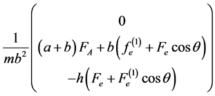
Computing the Lagrangian components  of the vector of forces in the tangent space and taking the projection
  (see (6)), one can check that the term to add to the right-hand side of (7), first three equations, is
The conclusion of Statement 1.1 about existence and uniqueness is not altered, since the matrix A of (12) is still the same.
Let us investigate about the effect of stabilization by the external device in the case of the force in A only:  (actually the overlap of
  does not change the substance). Moreover,
  has to vanish at the equilibrium:
 (20)
(20)
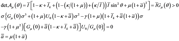
It can be easily seen that the characteristic polynomial (17) changes into
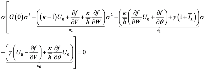 (21)
(21)
where the partial derivatives are calculated in . The following Proposition sets a selection of choices for f.
Proposition 1.2 (o) If  then the system is unstable.
1) for :
:
a) if  or
or  then the system is unstableb) if
  and
and  and
and  [resp.
 ], then the system is unstable [resp. stable].
2) For :
:
c) if  or
or , then the system is unstabled) if
  and
and , then the (real or complex) eigenvalues different from zero have negative real part.
Proof.
(o) Call . If
. If , then
 : since
 , a real positive eigenvalue certainly exists.
1) a) If  then at least one real negative eigenvalue
 ![]() exists and p can be written as
exists and p can be written as
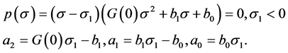 (22)
(22)
If , then
 : since
 , the equation
  has either two real positive solutions or two complex solutions with positive real part
 . Likewise, if
 , then it must be
  and we conclude in the same way.
b) It has to be checked the sign of : from (22) we see that
  must solve

The latter equation has a unique positive [resp. negative] solution  if and only if
  [resp.
 ]. For
  we conclude as before; on the other hand, if
  the real part of the (real or complex) solutions of
 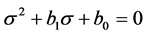 is negative.
2) c) If  then
then . The rest of the eigenvalues are the roots of
 . If
. If  then a real positive root exists, while if
  then either a real positive eigenvalue exists or the real part of the complex roots is positive.
d) In that case the eigenvalues are 0 (twice) and the two roots of , which are nonpositive if real or with nonpositive real parts if complex. □
The linear approximation  of (7) with the “new”
 ![]() encompassing the external force
encompassing the external force ![]() is
is  and
and
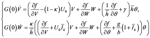 (23)
(23)
which generalizes (18). The partial derivatives are calculated at the equilibrium . The equation for
 ![]() replacing (19) is
replacing (19) is

(see (21) for the definition of![]() ,
,  ,
,![]() ). Hence the stable case 1), b) in Proposition 1.2 is asymptotic stability for
). Hence the stable case 1), b) in Proposition 1.2 is asymptotic stability for![]() . Case 2), d) concerns with
. Case 2), d) concerns with  so that
  (real or complex) and (assume
 )
)

where  comes from (23), second equation. Obviously each specific case (coincident eigenvalues,
  or
or ![]() equal to zero, ...) can be examined deeper.
equal to zero, ...) can be examined deeper.
Remark 1.5 A simple guess for f is , with
  and
and ![]() constant: in that case
constant: in that case  or
or  gives instability. The stability region located by case 1), b) in the quarter
 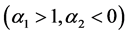 is not empty:
actually,  and
and  corresponds to the set
 , possibly cut on the upper part by the line
 , if the latter value is lower than
 . Such a set has a nonempty intersection with
 : indeed, it is sufficient to take, for each fixed
 ,
,  large enough in module.
Furthermore, the case 2), d) is simply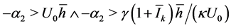 .
.
Inversely, the achieved conditions can be also read in terms of finding , for a given external force
 ![]() as in (20), in order to get stability. In particular, the case
as in (20), in order to get stability. In particular, the case  studied in [6] concerns with a counterbalance effect, so that the term UV in (7), second equation, vanishes.
Remark 1.6 The simplyfing assumption  sometimes used in models makes sense only around the equilibrium position: far from
  the linear approximation U constant would force the system to non reasonable predictions. Besides that, the same assumption is not a consequence of the equations, as we pointed out in Remark 1.1.
2. A Two-Body Model
2.1. The Equations of Motion
We now consider a rigid device simulating the front wheel, adding to the body  a rigid part
  (say the front wheel together with handlebars) hung in A and forming the angle
  (front steering) between the direction
 ![]() and a direction fixed in the body frame
and a direction fixed in the body frame :
:

For the sake of simplicity, we may imagine ![]() as a rigid bar laying on
as a rigid bar laying on![]() , with no active force operating on it. We now consider the five lagrangian coordinates
, with no active force operating on it. We now consider the five lagrangian coordinates . The angular velocity of
 ![]() is hence
is hence .
.
The Lagrangian function of the whole system is , where
 ![]() is the same as (1) and
is the same as (1) and

where  is a new lagrangian coordinate and
  and
and  are respectively the mass of
 ![]() and the central inertial momentum of
and the central inertial momentum of ![]() with respect to the direction
with respect to the direction . The equation of motion with respect to
  is simply
 (24)
(24)
Equation (24) gives

where  is the angle between
  and
and![]() .
.
Remark 2.1 If no further constraints are enjoined, the system is unstable the same: actually, changements in (7) are not essential: still keeping ,
,  is again an equilibrium point for the system
 , where


and (13), (17) are replaced respectively by
which has in the same way one real positive solution.
We now add the kinetic constraint of no skidding of ![]() at
at :
:  which gives
 (25)
(25)
A possible way to face the problem is to neglect the mass  of the anterior part, so that the Lagrangian function is the same as (1). However, a complication is, in our point of view, the role of
 , which does not appear in
![]() , but only in the constraint (25).
, but only in the constraint (25).
This is a nontrivial point for the theory-building of the correct equations of motion: the way we are going to follow is not to neglect the mass  and consider
 ![]() as the Lagrangian function. Even more, if we think of the problem as a “bicycle'” model, the front mass is not at all unsignificant for the overall frame.
as the Lagrangian function. Even more, if we think of the problem as a “bicycle'” model, the front mass is not at all unsignificant for the overall frame.
We now consider the set of Lagrangian coordinates : system (3) of the first kind Lagrangian equations is now replaced by the seven equations
 (26)
(26)
where![]() ,
, ![]() ,
, ![]() ,
, ![]() ,
,  ,
,  and
and ![]() are the seven unknown quantities. Concening with the initial conditions for (26) we can choose, with no loss in generality:
are the seven unknown quantities. Concening with the initial conditions for (26) we can choose, with no loss in generality:

Let us change for the sake of convenience  into the variable
 (27)
(27)
so that . The velocities
  are not independent, because of (2), (25): if on the one hand
  and
and  are arbitrary, on the other hand once
  has been fixed the initial velocities
 (28)
(28)
are imposed. In order to reduce (26) and eliminate the multipliers, we define, similarly to (4), the pseudovelocities
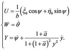 (29)
(29)
Joining (29) with (2) and (25), the lagrangian velocities  are written in terms of the parameters
 :
:
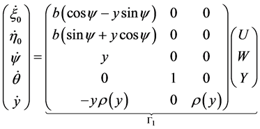
where  and, we recall,
 .
.
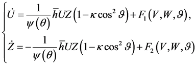
The equations of motion replacing (7) are now ,
,  together with (2), (25) and (29): straightforward computations lead to
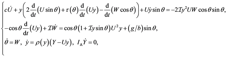 (30)
(30)
 (31)
(31)
where
 (32)
(32)
and, as before,  ,
,  ,
,  ,
,  ,
, .
.
Even in this case the equations of motion can be led back to the cardinal equations: indeed, calling  the rigid part containing A, B and
 ![]() (30), the second cardinal equation of the whole system
(30), the second cardinal equation of the whole system  using B for calculating the momenta and projecting along
  writes
 (33)
(33)
where  is the momentum of the external forces of the whole system. Since the constraints are smooth, the force in
  realizing the kinetic constraint (25) can be modelled as

so that (see also (10)) . On the other hand, the first cardinal equation for the whole system along
 ![]() is
is  Carring out all the computations, here omitted, one gets exactly (33). The second equation in (30) is again ascribable to the momentum balance of the system along
![]() , similarly to what discussed in Remark 1.1:
, similarly to what discussed in Remark 1.1:

Finally, the fourth equation in (30), namely (24), is simply the second cardinal equation written only for ![]() and with respect to the point
and with respect to the point , where all the momenta of the external forces vanish.
As we already remarked in Section 1, the overview of the system in the frame of the cardinal equations does not determine any conserved quantity: the only evident one is the energy conservation

2.2. The Mathematical Problem
System (30), (31) consists of eight ODEs for the eight variables![]() ,
, ![]() ,
, ![]() ,
, ![]() ,
, ![]() ,
, ![]() ,
, ![]() ,
, . The five equations (30) form a sub-system for
  together with the initial conditions
 (34)
(34)
while the constant value Y is deduced from (24), (27) and (28)):
 (35)
(35)
Once (30) has been solved, (31) and (28) allow to solve![]() ,
, ![]() ,
,![]() .
.
As in the case of Section 1, we incidentally remark that, if  and Y as in (35) is solution of (30), then
 ,
,  is solution of the same system, as we expect.
Statement 2.1 For any set of data (34), (35) system (30) admits one solution.
Proof. System (30) can be concisely written as
 (36)
(36)
with  and
and
the normal form being  with
with
and

It is evident that the unique solution of (30) corresponding to the initial data ,
,  ,
, 
 ,
, ![]() is
is  and W,
 ![]()
![]() identically zero. We notice that no other solutions such that the plane
identically zero. We notice that no other solutions such that the plane  is vertical are possible:
Statement 2.2 If , then
 ,
,  ,
,![]() . Conversely, if
. Conversely, if ,
,  and
and ,
,  ,
, ![]() , then
, then .
.
Proof. Set ![]() in (30) and call
in (30) and call :
:

The first two equations give ; on the other hand, eliminating
  from second and third equations yields
 , hence
  and
and . But
. But ![]() is consistent with the second equation only if
is consistent with the second equation only if  and the third equation leads to
![]() .
.
Conversely, if ,
,  ,
, ![]() are replaced in (30), one gets
are replaced in (30), one gets  that, together with the initial conditions, gives
![]() . □
. □
Still concerning with the initial data assignment, we notice that if  (which is a reasonable condition for
![]() ) we get from (35)
) we get from (35) : we wonder whether solutions such that
  (meaning
  and
and  constant) are possible. From (30), fourth equation, one gets
 ,
, . If
. If  we clearly have
 ,
,  and
and  for
for . If on the other hand
 , by replacing
  and
and ![]() in the first two equations of (30) we achieve the first integrals
in the first two equations of (30) we achieve the first integrals

so that only ,
, ![]() can be a solution. Substituting in the first integrals we see that
can be a solution. Substituting in the first integrals we see that ,
,  , that is the stationary solution.
We are going to investigate the stability of the stationary solution.
Proposition 2.1 The equilibrium point ,
, ![]() of (36) is unstable.
of (36) is unstable.
Proof. The Jacobian matrix at the equilibrium is
whose eigenvalues are![]() ,
,  ,
, . The linearized system

gives


with ,
,  ,
, . □
. □
We remark that, as bigger is  as longer is the time when the planar body
  falls to the ground
 .
.
3. Discussing Some Specific Assumptions
It is evident that the stability of the system can be achieved by introducing an external force as in Paragraph 1.3: instead of replay such a theme, we prefer to discuss some assumptions recurring in literature which indeed semplify the mathematical problem.
First of all, let us see what happens if we let , known constant. If
  then
then  and the solution is
  (that is
 ) and
) and . The point
  draws the circle
 ,
, .
.
On the other hand, if , the angle
  can be calculated by (30), fourth and fifth equations, regardless of the rest of the system:
 (37)
(37)
By integrating one gets in terms of :
:

In any case, if (30) is accepted, the assumption U constant allows the immediate calculation of , irrespective of
 ![]() and
and![]() .
.
The same system (30) is worth considering together with the assumption, not uncommon in literature [2] [9] -[11] , . Actually, assuming
 ,
,  constant, would lead to the invariant quantity
  and, by integration,
 . Hence also
 ![]() is proportional to
is proportional to ![]() and (30), second equation, can be written in terms of
and (30), second equation, can be written in terms of ![]() only:
only:

On the other hand, also (30), first equation, turns out to be written in terms of![]() , since
, since  and
and : it should be checked that two obtained equations show compatibility.
Hence, in our mind the angle  also must be governed by the equations of motion which do not make room for an assumption such as
 .
.
Nevertheless, assume that the mass of  is negligible, so that
  and
and , as it is found in some models: in that case fourth and fifth equations in (30) have to be disregarded and
  cannot longer be computed by means of (37). Following this point of view, the system is not closed, since
  enters only the constraint condition (25) and not in the Lagrangian function
![]() . This is the reason why an additional condition (say a constitutive law) is needed, as for instance
. This is the reason why an additional condition (say a constitutive law) is needed, as for instance .
.
References
- Gantmacher, F.R. (1975) Lectures in Analytical Mechanics, MIR.
- Astrom, K.J., Klein, R.E. and Lennartsson, A. (2005) Bicycle Dynamics and Control: Adapted Bicycles for Education and Research. Control Systems, IEEE, 25, 26-47. http://dx.doi.org/10.1109/MCS.2005.1499389
- Fajans, J. (2000) Steering in Bicycles and Motorcycles. American Journal of Physics, 7, 654-659. http://dx.doi.org/10.1119/1.19504
- Schwab, A.L., Meijaard, J.P. and Kooijman, J.D.G. (2012) Lateral Dynamics of a Bicycle with a Passive Rider Model: Stability and Controllability. Vehicle System Dynamics, 50, 1209-1224. http://dx.doi.org/10.1080/00423114.2011.610898
- Schwab, A.L., Meijaard, J.P. and Papadopoulos, J.M. (2005) Benchmark Results on the Linearized Equations of Motion of an Uncontrolled Bicycle. KSME International Journal of Mechanical Science and Technology, 19, 292-304. http://dx.doi.org/10.1007/BF02916147
- Ambrosi, D. and Bacciotti, A. (2009) Stabilization of the Inverted Pendulum on a Skate. Differential Equations and Dynamical Systems, 17, 201-215. http://dx.doi.org/10.1007/s12591-009-0016-8
- Ambrosi, D. and Bacciotti, A. (2007) The Bicycle Stability as a Control Problem. Politecnico di Torino, Rapporto interno n. 33.
- Braun, M. (1978) Differential Equations and Their Applications. Springer-Verlag, New York.
- Ambrosi, D., Bacciotti, A. and Ropolo, G. (2008) La matematica della bicicletta. La Matematica nella Società e nella Cultura I, Serie I, 477-492.
- Doria, A., Formentini, M. and Tognazzo, M. (2012) Experimental Analysis of Rider Motion in Weave Conditions. Proceedings Experimental and Numerical Analysis of Rider Motion in Weave Conditions, Vehicle System Dynamics, 50, 1247-1260. http://dx.doi.org/10.1080/00423114.2011.621542
- Lowell, J. and McKell, H. D. (1982) The Stability of Bicycles. American Journal of Physics, 50, 1106-1112. http://dx.doi.org/10.1119/1.12893