Open Journal of Modern Hydrology
Vol.3 No.4(2013), Article ID:38885,12 pages DOI:10.4236/ojmh.2013.34026
Application of Synthetic Meteorological Time Series in BROOK90: A Case Study for the Tharandt Forest in Saxony, Germany
![]()
1Meteorology, Technische Universität Dresden, Dresden, Germany; 2Mathematical Modelling, Bauman Moscow State Technical University, Moscow, Russia.
Email: *rico.kronenberg@tu-dresden.de
Copyright © 2013 Kronenberg Rico et al. This is an open access article distributed under the Creative Commons Attribution License, which permits unrestricted use, distribution, and reproduction in any medium, provided the original work is properly cited.
Received September 1st, 2013; revised October 1st, 2013; accepted October 8th, 2013
Keywords: Richardson Model; Weather Generator; BROOK90; Synthetic Time Series; LARS-WG; Forest Water Balance; Taylor Diagram; Cumulative Periodogram
ABSTRACT
This study presents an extended version of a single site daily weather generator after Richardson. The model is driven by daily precipitation series derived by a first-order two-state Markov chain and considers the annual cycle of each meteorological variable. The evaluation of its performance was done by deploying its synthetic time series into the physical based hydrological model BROOK90. The weather generator was applied and tested for data from the Anchor Station at the Tharandt Forest, Germany. Additionally its results were compared to the output of another weather generator with spell-length approach for the precipitation series (LARS-WG). The comparison was distinguished into a meteorological and a hydrological part in terms of extremes, monthly and annual sums and averages. Extreme events could be preserved adequately by both models. Nevertheless a general underestimation of rare events was observed. Natural correlations between vapour pressure and minimum temperature could be conserved as well as annual cycles of the hydrological and meteorological regime. But the simulated spectrums of extremes, especially, of precipitation and temperature, are more limited than the observed spectrums. While LARS-WG already finds application in practice, the results show that the data derived from the presented weather generator is as useful and reliable as those from the established model for the simulation of the water balance.
1. Introduction
The planning, construction and management of precipitation related infrastructure like sewer systems, retention areas or dams highly depend on the occurrence and statistical return period of extreme rainfall events [1,2]. In practise, robust and long time series for simulation and extrapolation of these events are needed to identify and consider such extremes. Hence, the lag of satisfactory long term observations leads to the development of stochastic models which are able to simulate rainfall without the recognition of atmospheric driven processes [3,4]. Their outcomes, long synthetic rainfall series, fulfil the requirements of the engineers. Thus, these models were extended with other meteorological variables and soon the first weather generators were presented [5]. These can be classified into Markov chain, spell length and non-parametric models [6,7]. The main disadvantage of these approaches is their limited capacity to model unobserved states as well as the incomplete preservation of statistical properties. They all depend on historical time series, which by definition can not include unobserved extremes of weather variables. In particular, they are not able to model non-stationary processes. But the transition from stochastic weather generators to stochastic nesting approaches or weather state models is possible. Therefore even changes of the climate can be recognized by integrating different scenarios [8,9] or by including a certain expected trend [10].
The great advantage of these generators is their speed unmatched by any other tool to simulate locally consistent future time series. They are very fast algorithms to produce long time series, which find a vast extent of applications as input in hydrological, hydrodynamic and other climate variable driven models [11-16].
The main focus in this study lies in the derivation and extension of the Richardson model and its application to observed data under the strict preservation of diurnal variations. More particularly not just the preservation of temporal properties was a major goal but also the physical consistencies between the considered meteorological variables. Here from arise the following motivational questions of this paper:
1. Do the simulated empirical distributions of meteorological elements fit the observed ones in terms of rare events (i.e. extremes)?
2. Are physical correlations of the water balance preserved by the weather generators?
3. Are the approaches able to retain the annual cycles of the considered hydrological and meteorological elements?
In the tradition of weather generators two philosophies were compared for single site time series in terms of a certain location, a Markov chain with a spell length model. The physical consistencies were investigated by deploying the simulated time series into the hydrological model BROOK90 [17].
2. Data and Study Region
2.1. Tharandt Forest
The Tharandt Forest is situated 20 km south west of Dresden and forms a part of the north eastern boundary of the eastern Ore Mountains. The forest spans a territory of 6000 ha [18], whose extent is shown in Figure 1. It is the largest contiguous area of forest dominated land use in Saxony, Germany. In average the territory is located 350 to 400 m asl and therefore features just a small relief intensity [19]. The highest point is the Tännicht with 461 m asl and the lowest is located in Coßmannsdorf with 197 m asl. The area forms a distinct cuesta in the north, which is a boundary to the Mulde loess hills and in the east a boundary to the eastern foothills of the Ore Mountains [20-22].
Due to its location near the north-eastern ridges of the Ore Mountains the study area shows an increased continental character of the climate in contrary to the western parts. Hence, the observed climate is representative for the climatic conditions of the foot hills of the eastern Ore Mountains. Though, the dominance of the forested land in combination with the local topography lead to significant differences from the regional climate conditions [23]. However, the bimodal distribution of the mean annual precipitation also can be observed, which is distinctive for this region.
2.2. Meteorological Data
The meteorological time series were observed at the An-
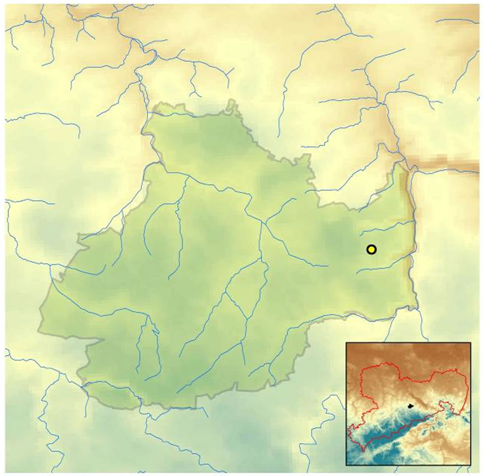
Figure 1. Tharandt Forest with Anchor Station (50˚58'N, 13˚34'E, 385 m asl) and altitude in m asl; the Wildacker Station is nearby located.
chor Station (50˚58'N, 13˚34'E) in the Tharandt Forest, Germany. The elements include precipitation, solar radiation, vapour pressure, average, minimum and maximum temperature. They are measured by the Chair of Meteorology at Technische Universität Dresden since the late 1950s. The time series used here is from 01/01/1997 until 09/30/2009 in daily resolution; it reflects the start of continuous flux measurements of, e.g. evapotranspiration at the site [24]. The time series were checked for stationarity, homogeneity and data gaps. The quality assessment was done considering the measurements at the nearby meteorological station Wildacker, which served as reference station. Hence, non-stationarities and heterogeneity could be excluded and no data gaps were found [25]. Further corrections of precipitation measurements were omitted [26,27]. The aforementioned bimodal distribution of the monthly mean precipitation of the Wildacker Station can be seen in Figure 2. It summarizes the climatic conditions from 1971 to 2010 at the site.
3. Methods
Stochastic models often find application in hydrology and meteorology as they offer the possibility to generate long and persistent time series.
The main reason for this frequent usage is the short availability of sufficient long and complete observed
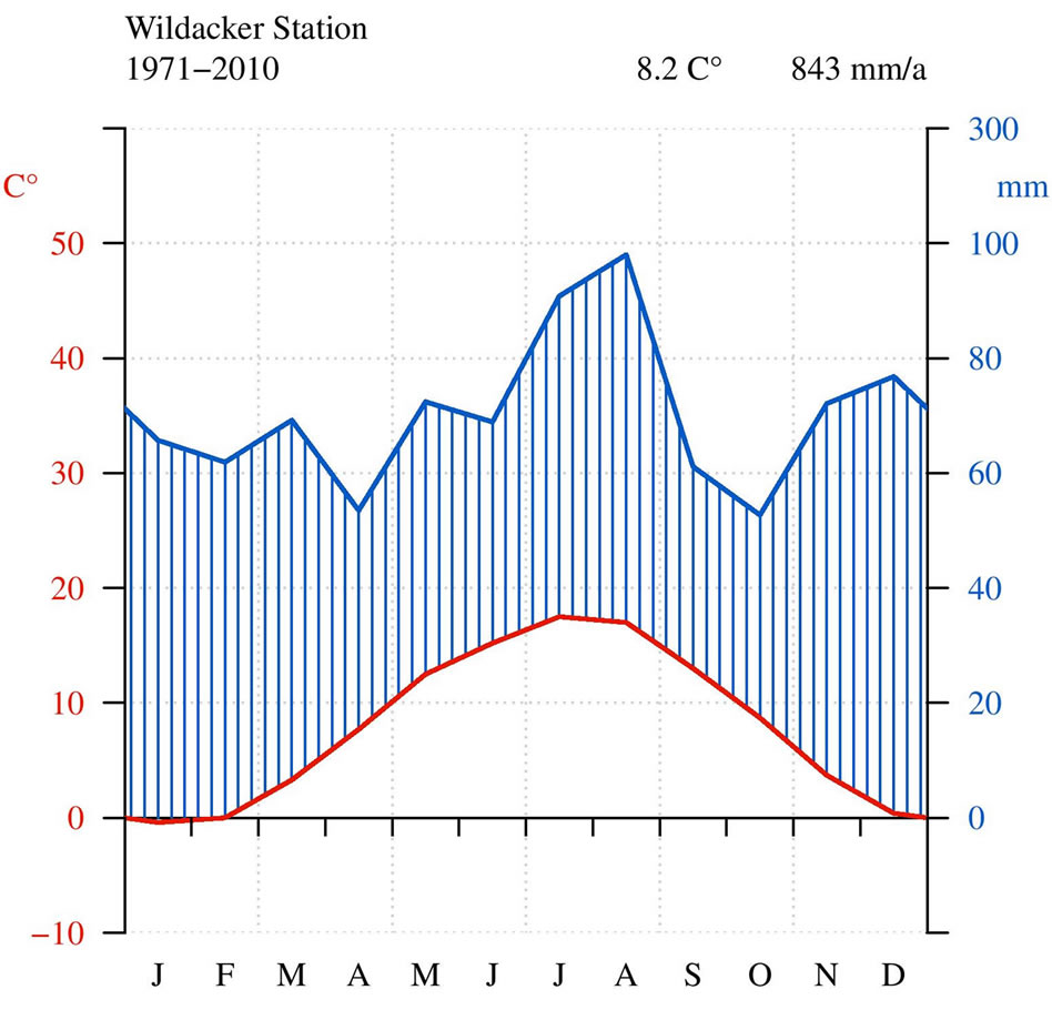
Figure 2. Climate diagram after Walter and Lieth [28] of the Wildacker Station nearby the Anchor Station in the Tharandt Forest for the period from 1971 until 2010.
time series.
Stochastic models enable to fill gaps in observed series of meteorological variables and to generate synthetic time series without actual time reference but unlimited length. These kinds of models are commonly called “weather generators”.
On the one hand a type of model, often deployed is the aforementioned “spell-length” approach. Time series are simulated by the addition of dry and wet periods according to the distribution of such periods in the observed data. The daily amount of precipitation is often derived by parametric distribution function of precipitation (e.g. gamma, log-Gaussian or mixture distributions). On the other hand so called Markov chain models are approaches which are often applied. It is possible based on observation to describe precipitation as stochastic process. These processes are of such a kind that occurrence probabilities of precipitation depend on a finite number of former days. After the generation of wet or dry days the amount of precipitation is similar to the spell-length models derived by aforementioned distribution functions. Richardson introduced a model which extended the synthetic precipitation series with other meteorological elements. Further the applied extended Richardson model is presented for the single site simulation of meteorological variables. All used symbols are summarized in Table 1.
3.1. Extended Richardson Model-ERM-Precipitation Estimation
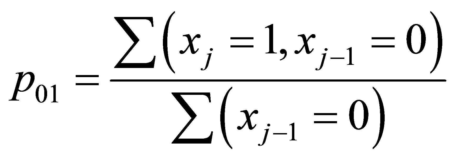
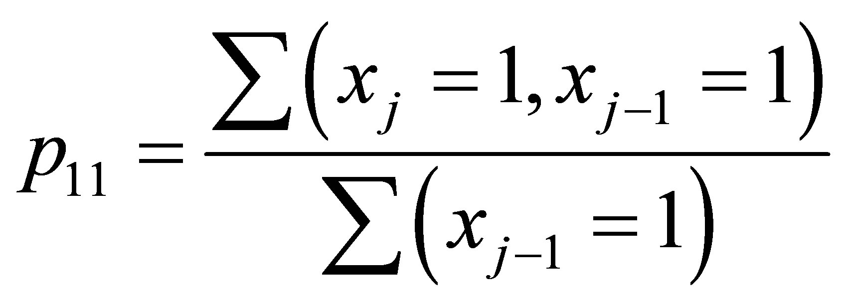
Precipitation was modelled through a first-order twostate Markov chain for a single station. The stochastic process model is called first-order because the probability if today is a wet day just depends on yesterday. More time lags would increase the order. Likewise it is a two state model which means that just wet or dry states are considered. The conditional probabilities for wet after dry and wet after wet days can be calculated according to Equations (1) and (2), which are based on binary coded series x of wet and dry days. Therefore the shown summations of all j observed days with the defined restriction have to be calculated.
 (1)
(1)
 (2)
(2)
Random numbers u and v are normally distributed with zero mean und standard deviation one.
 (3)
(3)
After the determination of the conditional probabilities they were used in combination with the generated random numbers to simulate new binary series  of wet and dry states. This is done in the following manner. First an initial state has to be announced for the first day which would be the day’s probable condition
 . Second, according to Equations (4) and (5),
  changes from day to day in dependence of the generated random number u. Hence the daily conditions change according to the estimate transition probabilities.
 (4)
(4)
 (5)
(5)
Reference [29] used Fourier’s series to simulate day of the year (DOY) dependent transition probabilities (i.e.  and
and ). This recommendation seemed reasonable. Since, like shown in Figure 3, also for the presented case an annual cycle of the transition probabilities can be observed. The Fourier’s series and their coefficients are defined in Equations (6) and (7), and in Table 2. The equations are already concrete solutions of the presented case study. For, the periods are 365 and 183 days as it can be seen in Figure 3.
 (6)
(6)
 (7)
(7)
To fit Fourier’s series Equations (1) and (2) have to be solved in dependence of DOY. The resulting conditional probabilities are defined as  and
and . These are shown in Figure 3 as observed series.
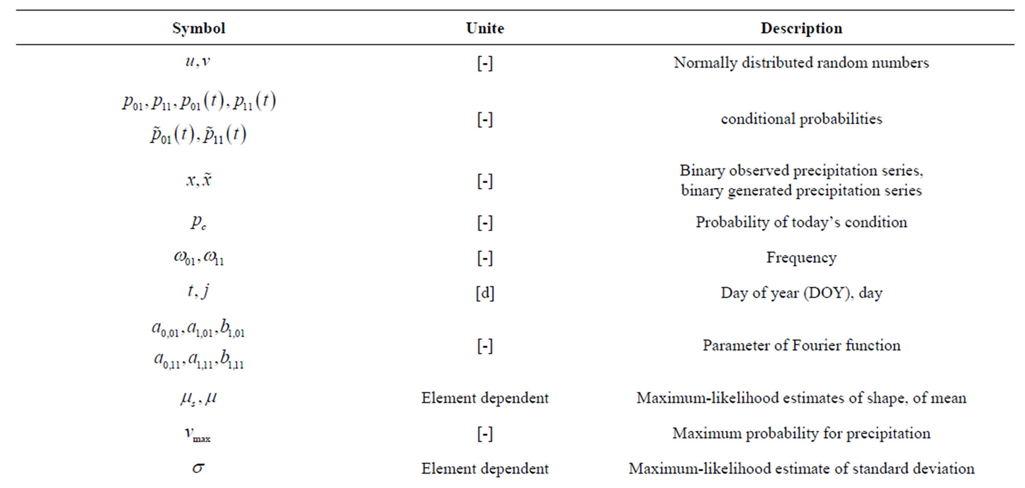
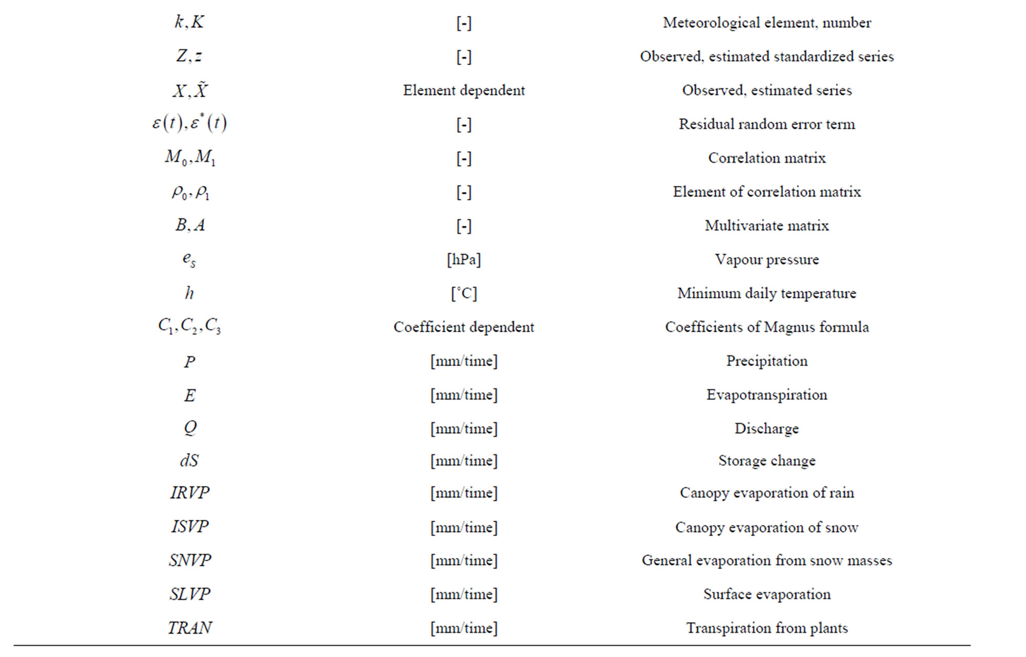
Table 1. Symbolism and nomenclature.
The coefficients  and
and  can be seen there as well, for they simply form the arithmetic means of the observed series. Thus, they represent the constant series. Finally the Fourier’s series resulting from Equations (6) and (7) were deployed for the modelling.
The daily precipitation amount is calculated in dependence of the binary-coded wet dry series (i.e. ). As in Equation (8) defined an inverse gamma distribution was deployed. Its shape parameter
  was derived as maximum likelihood estimate for each month. The re-
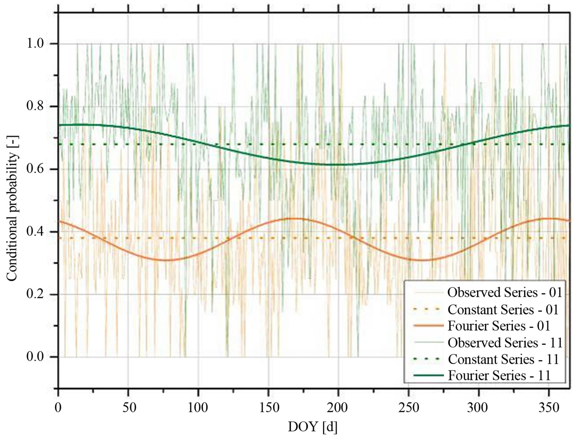
Figure 3. Different series of conditional probabilities in dependence of DOY for the deployed data sets of the Anchor Station, Tharandt.
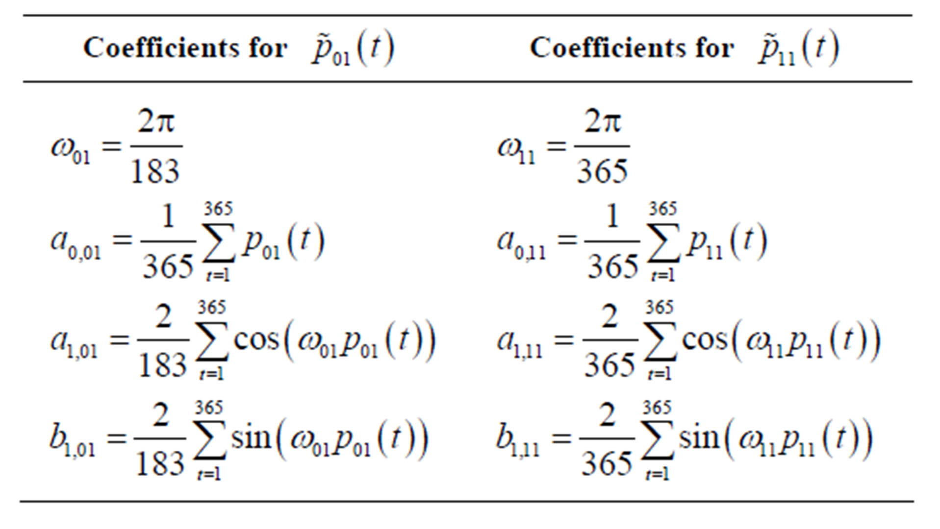
Table 2. Frequencies and coefficients of the deployed Fourier’s series to model in dependence of DOY conditional probabilities of wet and dry days.
sults are concluded in Figure 4 of all estimated monthly distributions.
 (8)
(8)
3.2. Extended Richardson Model-ERM-Estimation of Other Meteorological Elements
The other meteorological elements depend on the generated precipitation series, precisely on the binary coded wet and dry state series![]() . First the observed series
. First the observed series  were standardized according to Equation (9) over all variables k.
 (9)
(9)
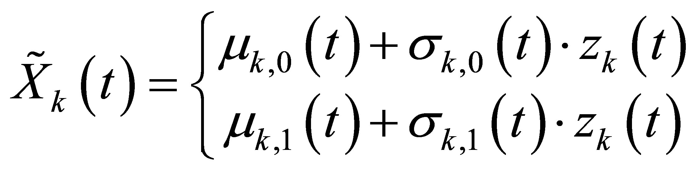
The new estimated meteorological series  then simply depend on the daily conditions (i.e. wet = 1 or dry = 0) and the estimated DOY (i.e. t = DOY) dependent mean and standard deviation like defined in Equation (10).
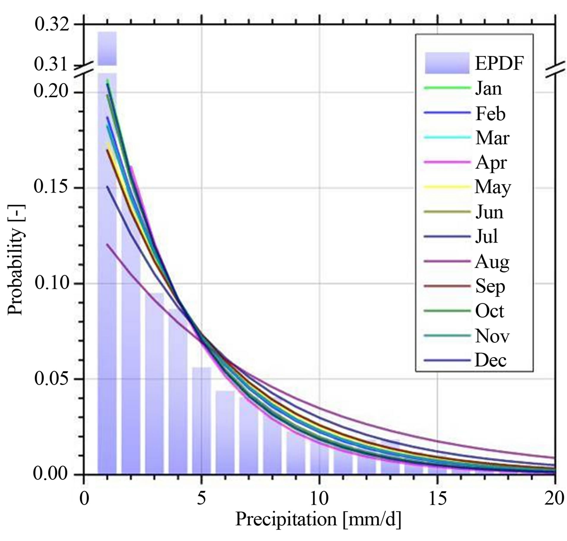
Figure 4. Empirical and theoretical distribution functions (i.e. 1 mm bins) of daily precipitation for the Anchor Station, in bars depicted are the annual empirical distribution function (EPDF) of the Anchor Station for the observed period.
 (10)
(10)
The standardized series 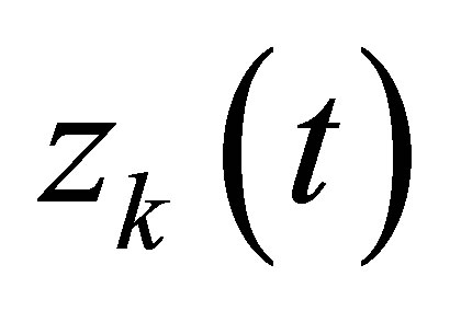 depend on the state the previous day, two multivariate matrices and a residual random error term, like shown in Equation (11).
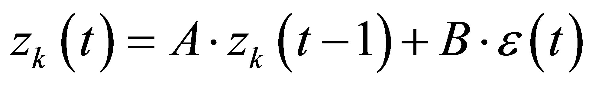 (11)
(11)
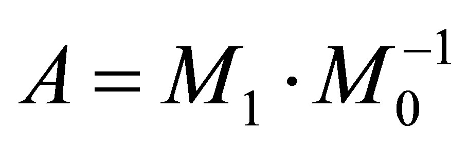
The multivariate matrices A and B are defined in Equations (12) and (13). B has to be calculated through Cholesky or Q/R decomposition [30] .
 (12)
(12)
 (13)
(13)
M1 and M0 are lag-zero and lag-one cross correlation matrices, with elements defined in Equations (14) and (15):
 (14)
(14)
 (15)
(15)
The residual random error term is defined in Equations (16) and (17).
 (16)
(16)
 (17)
(17)
3.3. LARS-WG
The stochastic weather generator LARS-WG was developed to simulate daily synthetic meteorological time series for single site [31]. Its latest version 5.0 enables the user to model the actual as well as the future climate. All simulations depend on the observed series from which the necessary model parameters for probabilities and correlations are derived. These were used to simulated synthetic series which are simultaneously randomly distributed. In contrast to the aforementioned extended Richardson approach LARS-WG uses a spell-length approach to derive precipitation series [6,12]. Than the daily precipitation amount is calculated according to semi empiric distribution. Annual cycles of the meteorological elements are considered by using Fourier functions [32]. Unfortunately LARS-WG in its used version is only able to model precipitation, evapotranspiration, minimum and maximum temperature as well as solar radiation. Hence, in contrary to the ERM wind speed and vapour pressure are missing variables.
3.4. BROOK90
The hydrological model BROOK90 was developed to simulate the vertical soil water movement and the evapotranspiration for a certain land surface at a daily resolution. The model is process-orientated and its parameters hold a physical meaning [17].
The model is a complex lumped-parameter model and follows a ‘less is more’ philosophy, which is characterized by a strong generalization of stream flow generation pathways but enough to compare it to observed time series. This generalization even goes further by ignoring aspects like hill slope hydrology and spatial distribution to focus on factors determining evapotranspiration.
For these reasons its design may serve the purpose of sensitivity analysis by the possibility to include or exclude certain soil water sub-models, which can be necessary to simulate plant growth, biogeography or global hydrology.
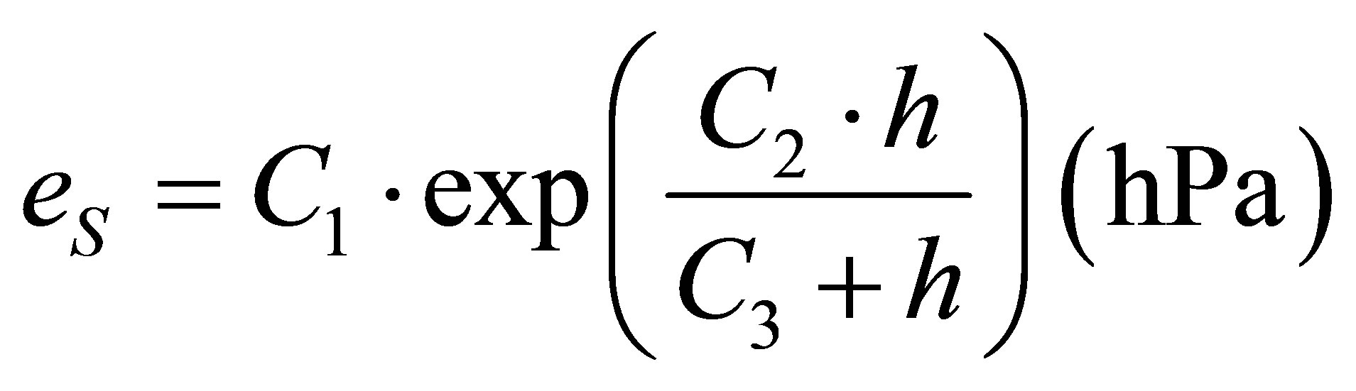
In consideration that LARS-WG does not estimate wind speed and vapour pressure the authors of BROOK90 suggest to work with a constant wind speed of 3 m/s and to calculate vapour pressure according to saturated vapour pressure. This was done using Magnus formula, which is defined in Equation (18).
 (18)
(18)
with over water: C1 = 6.1078 hPa; C2 = 17.08085;
C3 = 234.175˚C over ice: C1 = 6.1078 hPa; C2 = 17.84362;
C3 = 245.425˚C The necessary parameters were chosen according to the minimum temperature (i.e. <0˚C the surface was considered as ice), which was suggested by the BROOK90 authors.
The authors state that BROOK90 can fill a wide range of needs. It finds application in teaching and study water budget, water movement on small plots, evapotranspiration and soil water process. In addition it might answer questions related to land management and for the prediction of climate change effects. A further one was added to these tasks by deploying the model to validate the performances of weather generators.
The necessary model parameters of BROOK90 are taken from reference [25] (i.e. B2 configuration) which were determined for the considered period.
4. Results and Discussion
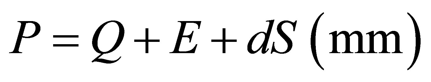
This study focuses on the extension and application of weather generators. Therefore the introductorily asked questions are of significant importance. The results where investigated from two perspectives to answer these questions. On the one hand meteorological properties are analyzed element wise by considering their correlations, periodicity and positive extremes (0.95 quantiles). On the other hand their hydrological properties are surveyed according to the long-term water balance defined in Equation (19). The precipitation (P) is defined as the sum of the discharge (Q), the evapotranspiration (E) and the storage change (dS). It is the water balance in its most common and most simple form [33].
 (19)
(19)
The results are four data sets, which are named and defined in the following manner: the observed (OBS), the extended Richardson model (ERM), the extended Richardson model without wind speed and vapour pressure (ERMw) and the LARS-WG data set (LARS). 1000 years long synthetic time series were simulated by each approach.
4.1. Meteorological Synthetic Time Series
First the correlations between minimum temperature and vapour pressure were investigated. Hence, the differences of simulated and calculated vapour pressure are outlined. The scatter plots are summarized in Figure 5. Figure 5(a) shows the natural correlations between minimum temperature and vapour pressure mainly following the generalization of Equation (18), with a not neglected scattering through natural fluctuation. The scattering becomes even broader between the simulated variables in Figure 5(b). But the physical correlations
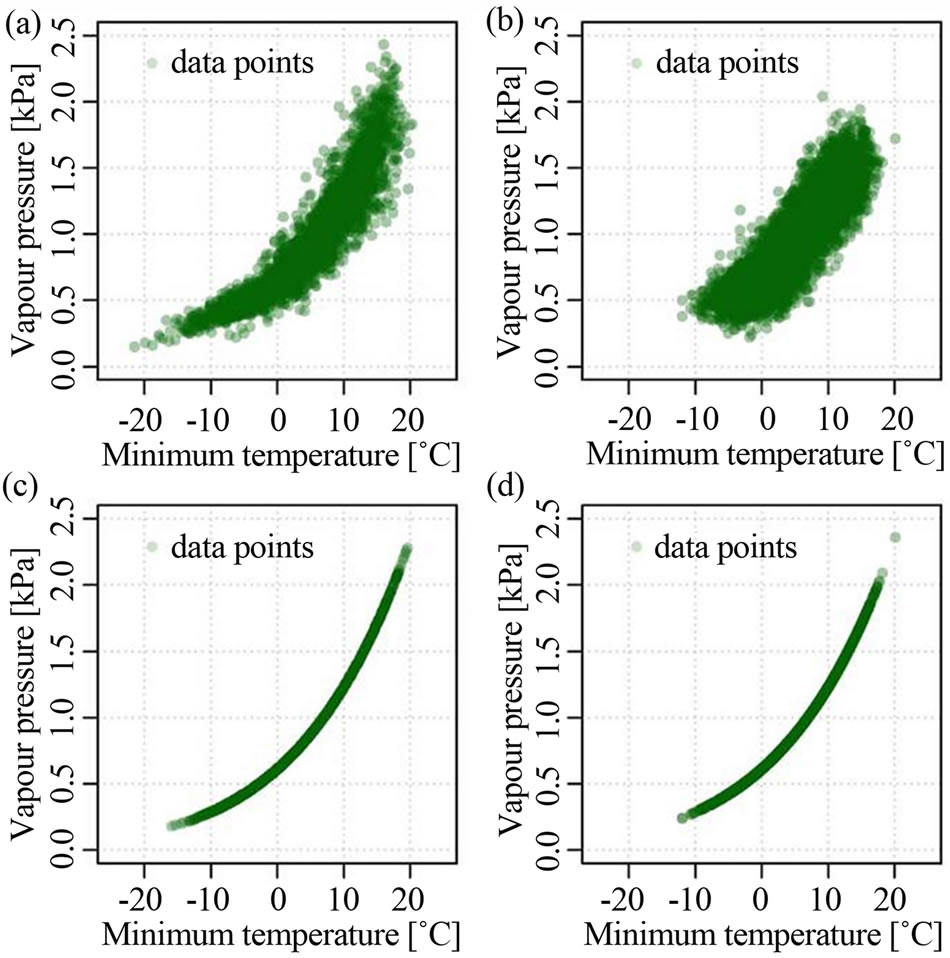
Figure 5. Correlations between minimum temperature and vapour pressure for 5000 randomly selected data points; (a) OBS; (b) ERM; (c) LARS; (d) ERMw.
and natural fluctuations could be preserved. Whereas Figures 5(c) and (d) show the curve of Equation (18) for LARS and ERMw, obviously these curves are the same.
The results of the investigations of the 0.95 quantiles are depicted in Figure 6. Compared are the Quantiles of simulated and observed variables. They give an insight on how the empirical distributions are located, especially the right tails of these distributions and how they match with the observed distributions. For all simulations, the quantiles of LARS as well as of ERM show a slight under estimation even independent of the season. With no regard on the approach the best fit can be observed in the vapour pressure. The wind speed is slightly better simulated by ERM than by LARS. Tough it must be stated that for LARS only a series of 3 m/s wind speed was generated. This unorthodox procedure arises from the recommendations of the BROOK90 authors. Nevertheless this value nearly represents the stations mean value.
The advantage of the applications of semi empiric distributions becomes obvious looking at the precipitation. The extremes of this meteorological element are better simulated by LARS than by ERM which just uses a gamma distribution.
The largest difference can be found between the simulated solar radiations, which so far cannot be explained.
No differences are observable between minimum and maximum temperature. The underestimations of these variables confirm the results in Figure 5, where the spectrum of possible values from minimum to maximum temperature is more limited, in contrast to the observed
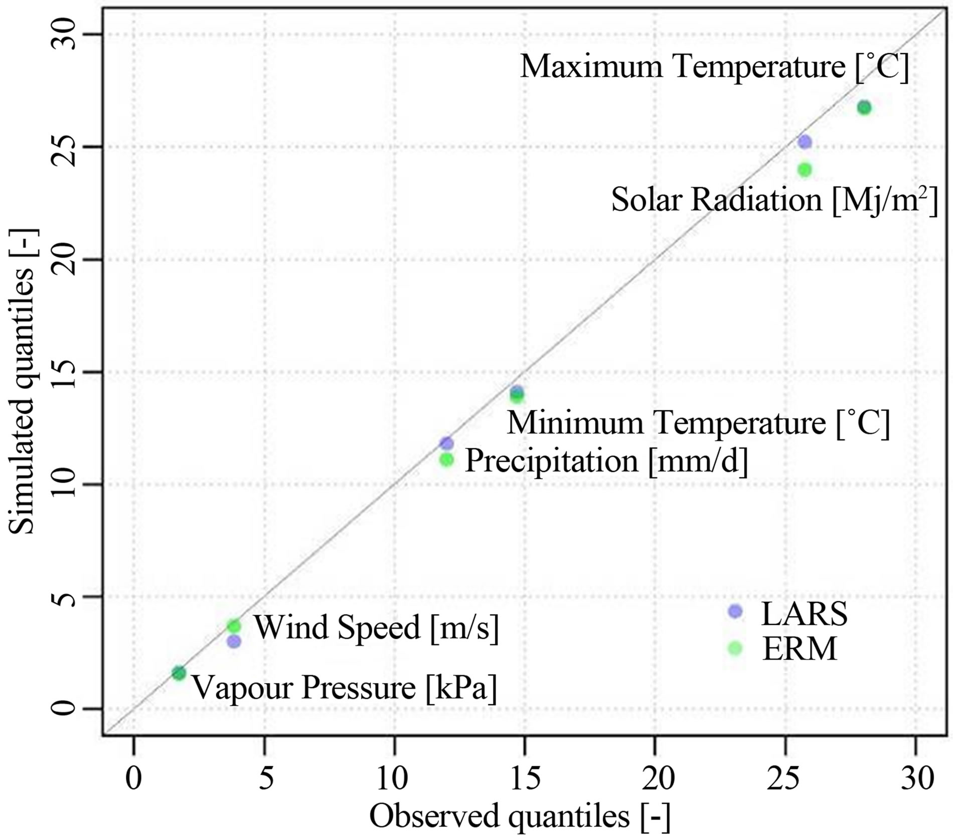
Figure 6. 0.95 Quantiles of all modelled variables for LARS and ERM simulations of 1000 years time series.
spectrum. Thus the tails of the simulated distributions are more limited.
Reference [34] stated that apart from the test of white noise a cumulative periodogram also can be used to examine hidden and suspected periodicities. In this context the monthly synthetic and partly observed time series of the meteorological variables were plotted in Figure 7. So a validation of their periodicity is qualitatively possible.
All variables of the observed and simulated series show a jump at a frequency of 0.0833 which is equivalent to 12 month (i.e. red highlighted in Figure 7). While all variables are characterized by a large significant jump at this point, precipitation follows more or less the 0.5:1 line. The simulated series of precipitation even shows signs of higher periodicity. These jumps just can be explained with the periodicity of months. As obvious also simple series of returning months (i.e. {1, 2, 3, …, 12, 1, ..}) are plotted and show significant steps.
These steps are also obvious in the monthly series of precipitation. There it can be explained by the fitting of distributions functions depending on the month (cp. Figure 4).
Figure 7 proves that all simulated variables of ERM follow an annual cycle. Even rather artificial inner annual periodicities caused by the model parameterisation of precipitation are preserved.
4.2. Long-Term Water Balance
The Taylor diagram was developed to illustrate the relation between correlations, standard deviation and root mean square error [36]. It is commonly applied for GCM validation. In this case instead of different models the water balance components are drawn in Figure 8. The
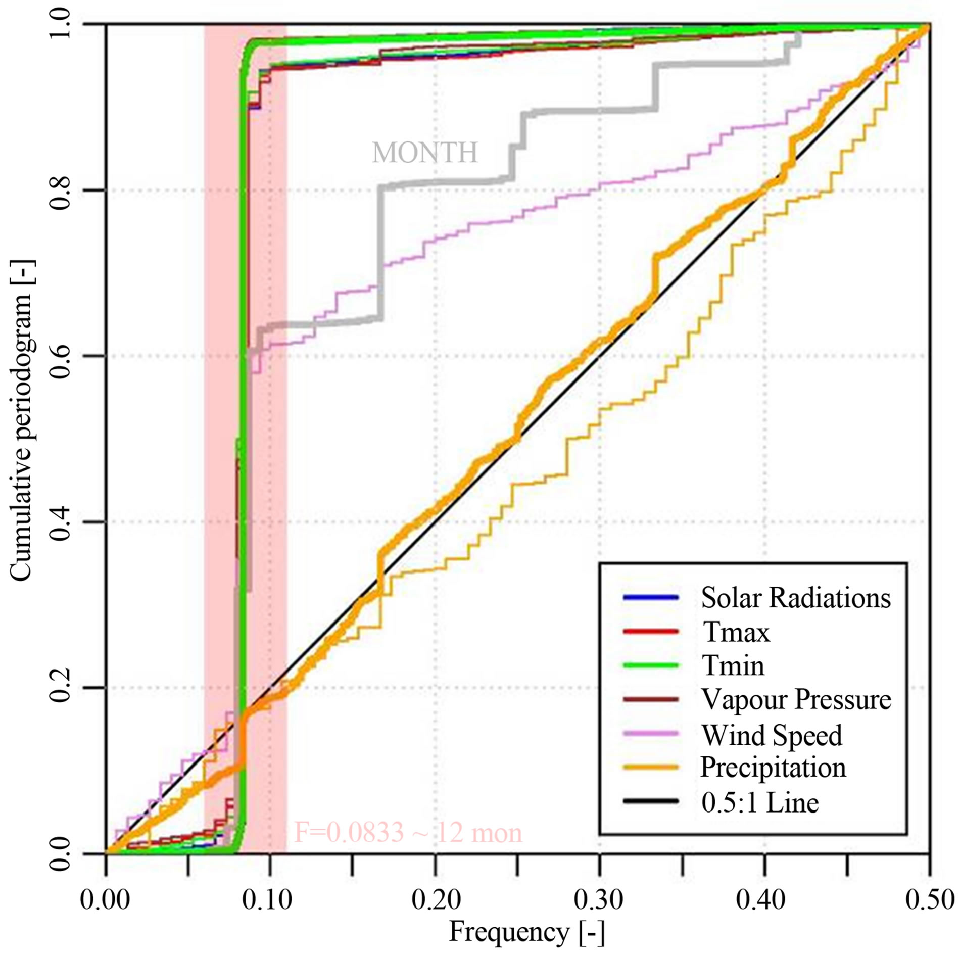
Figure 7. Cumulative periodogram [35] of monthly meteorological variables of OBS and ERM; depicted in bold lines is ERM and in thin lines OBS data.
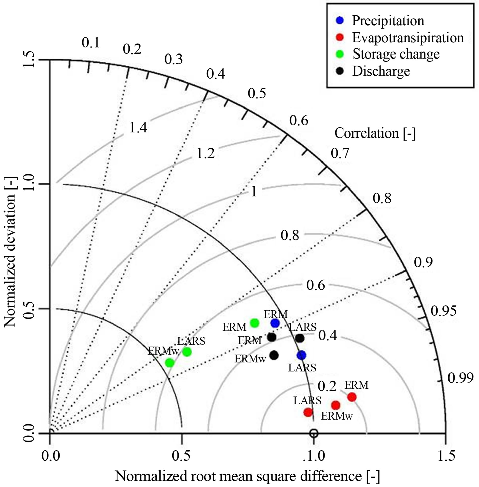
Figure 8. Taylor diagram of the monthly mean standardized values of the long-term water balance elements estimated for 1000 years periods for each model.
meaning remains the same as in its former usage; the closer a point lies to the reference at one on the abscissa the better or closer the simulated component behaves to the reference state (i.e. observed state).
The evapotranspiration could achieve the best results, consistently gaining a correlation higher than 0.99 with no dependence on the model. The LARS lies closest to the reference point followed by ERMw and ERM. But the differences are very small. Generally it can be stated that all models simulated the evapotranspiration really close to the observed state.
These results for ERM could only be achieved because of a post processing of the BROOK90 calculations. Negative E values in winter could be observed in the model runs driven by ERM data. BROOK90 calculates E according to Equation (20). The negative E resulted from negative values caused by the canopy evaporation of snow term (ISVP).
 (20)
(20)
To solve this contradiction of negative E values, ISVP was excluded from its calculation to obtain realistic results. Therefore the water balance had to be closed by the summation of the excluded term (i.e. ISVP) with Q. This post processing occurred to be necessary just for the ERM run. Unfortunately plausible reasons for this behaviour could not be figured out, since the physical correlations between minimum temperature and vapour pressure are preserved, as depicted in Figure 5(b). The authors of BROOK90 give a vague explanation of this particular behaviour by arguing that the canopy evaporation of snow is still a rather unknown process. Hence, its consideration in a hydrological model may lead to the observed uncertainties. Nevertheless, this post processing lead to reasonable results for ERM as Figures 8 and 9(b) conclude.
The differences at a monthly scale for the precipitation are larger. While LARS reaches a correlation of 0.95 ERM achieved fairly 0.89. However both results are outstanding compared to other investigations [37] where precipitation, because of its supposed randomness in time and space at this scale, is the most defficile element to simulate. The significant better performance of LARS can be explained by the usage of a semi empiric distribution for the modelling of precipitation, which obviously estimates the daily amount more precise.
Referring to the system’s output, the discharges are not wide spread in Figure 8. They lie between a correlation of 0.9 and 0.95. The best performance to the references is shown by ERMw followed by LARS and ERM.
The results of the residual storage change term, in contrast, scatter quite within the diagram, while both elements without estimated vapour pressure and wind lie closer to each other (i.e. LARS and ERMw) and their correlations are about 0.85. ERM lies apart from them, but nearer to the reference state. Thus the standard deviation of ERM is closer to the reference than those of the others. ERM is considered as best estimated of the storage change, even if its percentage of the overall water balance is marginal.
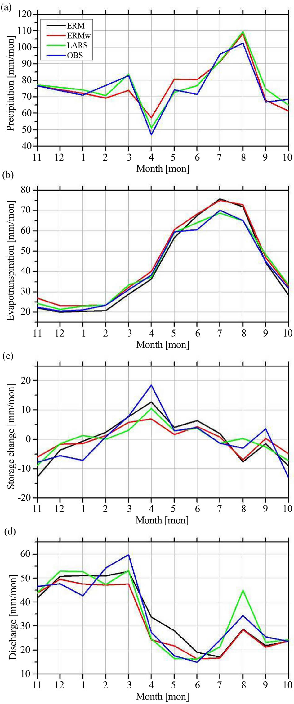
Figure 9. Monthly mean water balance components of 1000 years simulated time series of ERM, ERMw, LARS and OBS, (a) Precipitation; (b) Evapotranspiration; (c) Storage change; (d) Discharge.
The normalized standard deviations for all water components do not differ much from the reference states, except the peculiarities observed within the store change terms.
Hence, for each component of the water balance a certain model performs best, but in conclusion through the help of the diagram the best model could not be identified.
In Figure 9 the mean monthly diurnal variations of each component of the water balance are depicted. The precipitation shows no significant differences comparing the curves of the models. ERM and ERMw have the same precipitation curves as they just differ in their wind speed and vapour pressure series. LARS seems to be closer to the observed precipitation, as Figure 8 already indicates. The overestimation of precipitation by each model in March and August must be mentioned. In context of Figure 2, the month with the largest precipitation amount is always overestimated by the weather generators. The main reason for this may be the occurrence of the aforementioned rare extreme event in August 2002, which is included in the observed time series [25]. This event influences the weather generators to much, which lead to the consequent over estimation of summer precipitation.
The curves of the evapotranspiration are very close to the observed results, only ERM and ERMw overestimate evapotranspiration in the summer months about 5 mm, An explanation might be the oversupply of water and energy simulated by ERM in these months.
But the results are still satisfactory taking into account the aforementioned post processing for the ERM driven BROOK90 run.
The curves of the storage change are more distinguishable. The simulated results preserve the annual cycle as clearly depicted in Figure 9(c). The investigation of the curves in detail indicates that they have more in common among themselves than to the observed curve. This curve is characterized by a certain peak in April, most likely caused by the annual snow melting, which is indicating a certain limitation of the weather generators to reproduce these atmospheric conditions. This peak arises, with one month latency, from the melting in March, which clearly can be seen in Figure 9(d). Of further importance is the peak simulated by LARS in August, which results from the larger precipitation and less evapotranspiration in this month. Mainly it is caused by the aforementioned disproportional consideration of the known rare event in this month.
The annual water balance shows less significant differences as depicted in Figure 10. LARS and ERM in average overestimate all components of the water balance, whereby the differences are slightly higher for the LARS results. Despite ERMw behaves also as coherent as the other results it shows more distinguishable differences. The lowest uptake of water trough evapotranspira-
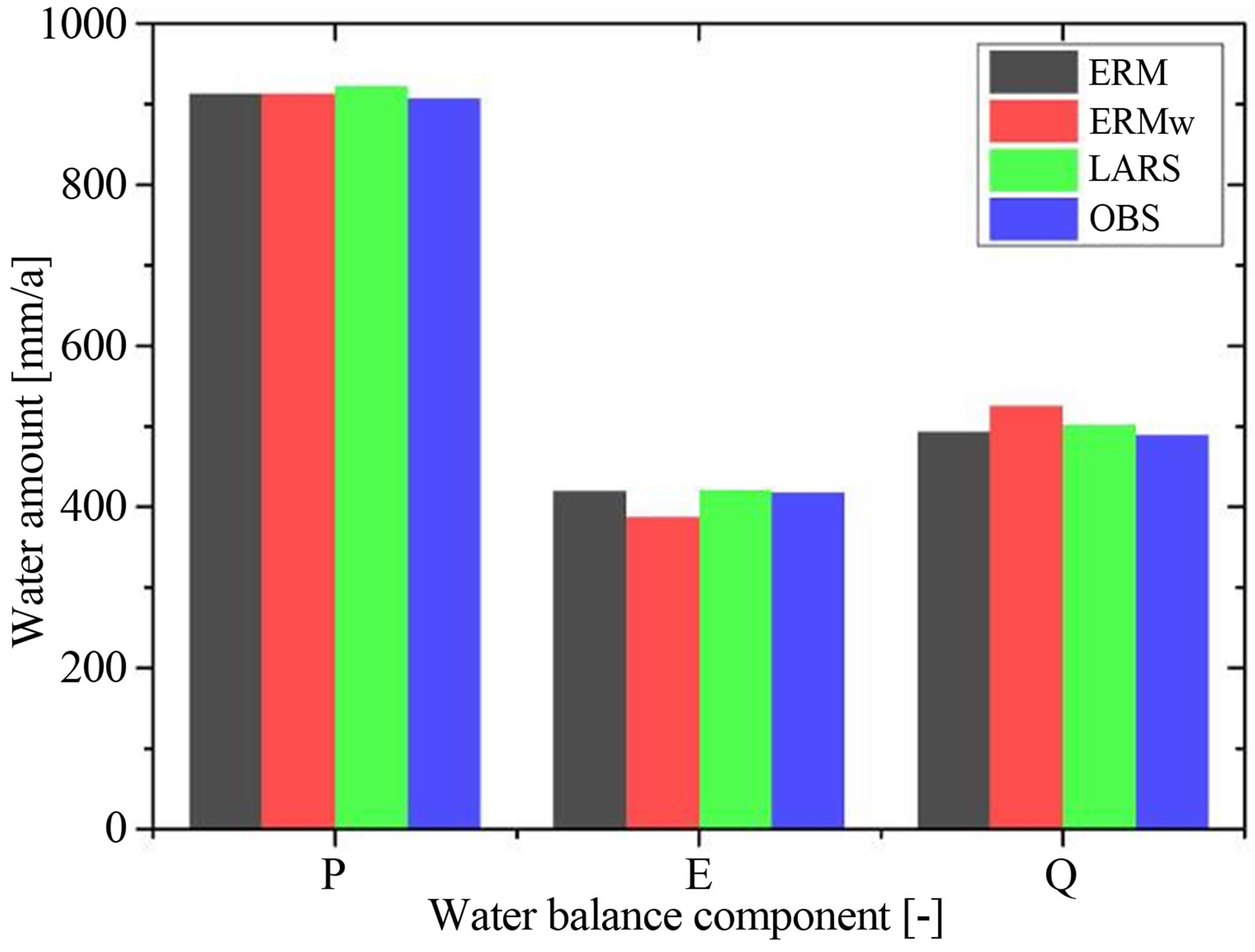
Figure 10. Annual mean water balance components of 1000 years simulated time series of ERM, ERMw, LARS and 12 years OBS.
tion leads to a larger system output by discharge in the catchment.
The differences are even clearer looking at Table 3. As already mentioned the deviations of ERM and LARS are neglectable small of <3%. ERM even reaches results of <1% deviation from the observed water balance. The aforementioned differences of ERMw can also be seen clearly. Additionally also the residual storage change term is given in Table 3. The observed value is rather small as expected, almost zero. According to this small absolute value are the differences large.
5. Conclusions and Outlook
In this study another extension of a Richardson based weather generator is presented. Its application to the hydrological model BROOK90 for the Anchor Station in the Tharandt Forest, Germany is discussed. To contextualize its results, the performance of the model was compared to another weather generator (i.e. LARS-WG).
Rare events of any considered meteorological element are well maintained. Though, LARS better performed in terms of precipitation due to the usage of a semi empiric distribution function. For this reason the application of mixture distributions or non-parametric distribution functions most likely will improve the presented weather generator [38].
Generally, only underestimations could be observed. Through the application of a cumulative periodogram it is proven that also the annual cycles are preserved. The analysis even shows a subtle visible influence of the chosen parameterization of monthly fitted distributions functions for precipitation. The natural correlations of minimum temperature and vapour pressure are sufficiently considered. Thus, through the underestimation of
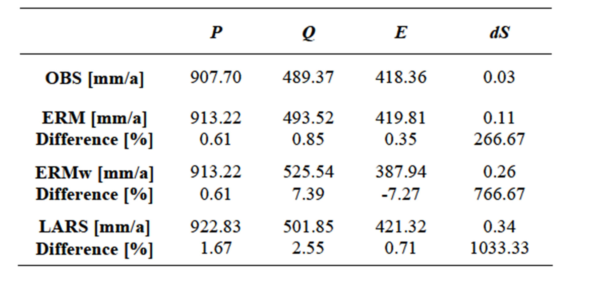
Table 3. Annual mean sums and differences of the water balances components of 1000 years long synthetic and 12 years long observed time series.
temperature extremes, the natural spectrum could not be covered completely neither by ERM nor by LARS.
The application of the weather generators in a hydrological context showed temporal and element wise dependences of the performance. While the simulated data set of LARS-WG shows better results for precipitation and evapotranspiration on a monthly basis, ERM performed better on the annual scale for these elements.
The application of ERM in BROOK90 resulted in a post processing due to implausible negative evapotranspiration values in winter, which were caused by a “canopy evaporation of the snow” term. The presented approach is a practical solution, but the authors would always prefer a better description and parameterisation of the responsible processes.
Overall the hydrological perspective emphasises the preservation of annual meteorological and hydrological regimes. Both applied models are useful and reliable for modelling the water balance.
The presented weather generator (i.e. ERM) could be extended from a single site to a raster-based multi site weather generator, which might be coupled with a cascade model for the downscaling from daily to 5 min time series [39]. However, this would require a change for the hydrological modelling to a raster based model like WaSimETH [37].
As a result of the related demands of information considering the future climate at a regional scale likewise the intention arose to simulate climate scenarios by the recognition of other future atmospheric properties like GCM outputs [40].
6. Acknowledgements
This work was supported by the German Academic Exchange Service (DAAD). Special thanks go to Dr. Uwe Spank and Dr. Klemens Barfus for helpful discussions, and Uwe Eichelmann and Heiko Prasse from the Chair of Meteorology at Technische Universität Dresden for their technical assistance.
REFERENCES
- DIN, “Drain and Sewer Systems outside Buildings,” Beuth-Verlag, Berlin, 2008.
- DWA, “Hydraulic Dimensioning and Verification of Drain and Sewer Systems,” Beuth-Verlag, Berlin, 2006.
- L. LeCam, “A Stochastic Theory of Precipitation. Proceedings of the 4th Berkley Symposium,” Mathematical Statistics and Probability, University of California Press, Berkley, 1961.
- K. R. Gabriel and J. Neumann, “A Markov Chain Model for Daily Rainfall Occurrences at Tel-Aviv,” Quarterly Journal of the Royal Meteorological Society, Vol. 88, No. 375, 1962, pp. 85-90. http://dx.doi.org/10.1002/qj.49708837511
- C. W. Richardson, “Stochastic Simulation of Daily Precipitation, Temperature and Solar Radiation,” Water Resources Research, Vol. 17, No. 1, 1981, pp. 182-190. http://dx.doi.org/10.1029/WR017i001p00182
- D. Wilks and R. Wilby, “The Weather Generation Game: A Review of Stochastic Weather Models,” Progress in Physical Geography, Vol. 23, No. 3, 1999, pp. 329-357. http://dx.doi.org/10.1177/030913339902300302
- J. P. Hughes, P. Guttorp and S. T. Charles, “A Non-Homogeneous Hidden Markov Model for precipitation Occurrence,” Applied Statistics, Vol. 48, No. 1, 1999, pp. 15-30. http://dx.doi.org/10.1111/1467-9876.00136
- H. Chen, J. Guo, Z. Zhang and C.-Y. Xu, “Prediction of Temperature and Precipitation in Sudan and South Sudan by Using LARS-WG in Future,” Theoretical and Applied Climatology, Vol. 113, No. 3-4, 2012, pp. 363-375. http://dx.doi.org/10.1007/s00704-012-0793-9
- A. Spekat, W. Enke and F. Kreienkamp, “New Development of Regional High Resoluted Circulation Patterns for Germany and Simulation of Regional Climate Scenarios with the Downscaling Model WETTREG on the Basis of Global Climate Simulations of ECHAM5/MPI-OM T63L31 2010 until 2100 for the SRES-Scenarios B1, A1B and A2,” Report, Umweltbundesamt, Berlin, 2007.
- B. Orlowsky, F.-W. Gerstengarbe and P. C. Werner, “A Resampling Scheme for Regional Climate Simulations and Its Performance Compared to a Dynamical RCM,” Theoretical and Applied Climatology, Vol. 92, No. 3-4, 2008, pp. 209-223. http://dx.doi.org/10.1007/s00704-007-0352-y
- M. Safeeq and A. Fares, “Accuracy Evaluation of ClimGen Weather Generator and Daily to Hourly Disaggregation Methods in Tropical Conditions,” Theoretical and Applied Climatology, Vol. 106, No. 3-4, 2011, pp. 321- 341. http://dx.doi.org/10.1007/s00704-011-0438-4
- M. A. Semenov, R. J. Brook, E. M. Barrow and C. W. Richardson, “Comparison of the WGEN and LARS-WG Stochastic Weather Generators for Diverse Climates,” Climate Research, Vol. 10, No. 2, 1998, pp. 95-107. http://dx.doi.org/10.3354/cr010095
- V. Y. Ivanov, R. L. Bras and D. C. Curtis, “A Weather Generator for Hydrological, Ecological, and Agricultural Applications,” Water Resources Research, Vol. 43, No. 10, 2007, pp. 1-21. http://dx.doi.org/10.1029/2006WR005364
- M. Khalili, F. Brissette and R. Leconte, ”Effectiveness of Multi-Site Weather Generator for Hydrological Modeling,” Journal of the American water resources Association, Vol. 47, No. 2, 2011, pp. 303-314. http://dx.doi.org/10.1111/j.1752-1688.2010.00514.x
- J. Xia, “A Stochastic Weather Generator Applied to Hydrological Models in Climate Impact Analysis,” Theoretical and Applied Climatology, Vol. 55, No. 1-4, 1996, pp. 177-183. http://dx.doi.org/10.1007/BF00864713
- C. W. Richardson, “Weather Simulation for Crop Management Models,” Transactions of the American Society of Agricultural Engineers, Vol. 28, No. 5, 1985, pp. 1602-1606.
- C. A. Federer, C. Vörösmarty and B. Fekete, “Sensitivity of Annual Evaporation to Soil and Root Properties in Two Models of Contrasting Complexity,” Journal of Hydrometeorology, Vol. 4, No. 6, 2003, pp. 1276-1290. http://dx.doi.org/10.1175/1525-7541(2003)004<1276:SOAETS>2.0.CO;2
- K. Mannsfeld and O. Bastian, “Landscape of Saxony— Catigorization of Manifold,” Landesverein Sächsischer Heimatschutz, Dresden, 2005.
- F. Haubrich, “The Tharandt Forest as Alegory of the Geology of Saxony,” Jahrestagung der Deutschen Bodenkundlichen Gesellschaft, Exkursionführer H5, Dresden, 2007.
- German Soil Science Society, “Soils without Borders— Anniversary of the German Soil Science Society, 02. bis 09. September 2007 in Dresden,” In: General Excursion Guide/ German Soil Science Society, 2007, Reports of the German Soil Science Society, Göttingen, 2007.
- P. Feger, K. Schwärzel, D. Menzer, C. Bernhofer, B. Köstner and F. Katzschner, “Anniversary of the German Soil Science Society—Soils without Borders, Dresden, Saxony, Germany,” Reports of the German Soil Science Society, Göttingen, 2007.
- H. Leser, “Diercke-Wörterbuch Allgemeine Geographie,” Westermann, Braunschweig, 2005.
- C. Bernhofer, “Exkursions-und Praktikumsführer Tharandter Wald. Material zum ‘Hydrologisch-Meteorologischen Feldpraktikum’,” Tharandter Klimaprotokolle 6, TU Dresden, Dresden, 2005.
- T. Grünwald and C. Bernhofer, “A Decade of Carbon, Water and Energy Flux Measurements of an Old Spruce Forest at the Anchor Station Tharandt,” Tellus B, Vol. 59, No. 3, 2007, pp. 387-396. http://dx.doi.org/10.1111/j.1600-0889.2007.00259.x
- U. Spank, K. Schwärzel, M. Renner, U. Moderow and C. Bernhofer, “Effects of Measurement Uncertainties of Meteorological Data on Estimates of Site Water Balance Components,” Journal of Hydrology, Vol. 492, 2013, pp. 176-189. http://dx.doi.org/10.1016/j.jhydrol.2013.03.047
- B. Sevruk, “Methodical Analysis of Systematic Measurement Errors of the Hellmann Rain Gauge for the Summer in Switzerland,” Versuchsanstalt für Wasserbau, Hydrologie u. Glaziologie, 1981.
- D. Richter, “Results of the Methodical Analysis of the Correction of Systematic Errors of the Hellmann Rain Gauge,” Selbstverlag des Deutschen Wetterdienstes, Offenbach am Main, 1995.
- H. Walter and H. Lieth, “Klimadiagramm-Weltatlas,” Gustav Fischer Verlag, Jena, 1967.
- J. Barron, J. Rockström, F. Gichuki and N. Hatibu, “Dry Spell Analysis and Maize Yields for Two Semi-Arid Locations in East Africa,” Agricultural and Forest Meteorology, Vol. 117, No. 1, 2003, pp. 23-37. http://dx.doi.org/10.1016/S0168-1923(03)00037-6
- N. Herrman, “Höhere Mathematik/für Ingenieure, Physiker und Mathematiker,” Oldenburg Verlag, München, Wien, 2007. http://dx.doi.org/10.1524/9783486593518
- M. A. Semenov and E. M. Barrow, “Use of a Stochastic Weather Generator in the Development of Climate Change Scenarios,” Climatic Change, Vol. 35, No. 4, 1997, pp. 397-414. http://dx.doi.org/10.1023/A:1005342632279
- M. S. Khan, P. Coulibaly and Y. B. Dibike, “Uncertainty Analysis of Statistical Downscaling Methods Using CGCM Predictors,” Hydrological Processes, Vol. 20, No. 14, 2006, pp. 3085-3104. http://dx.doi.org/10.1002/hyp.6084
- S. Dyck and G. Peschke, “Grundlagen der Hydrologie,” Verlag für Bauwesen, Berlin, 1995.
- K. W. Hipel and A. I. McLeod, “Time Series Modelling of Water Resources and Environmental Systems,” Elsevier Scientific Publishing Company, Amesterdam, 1994.
- G. E. P. Box, G. M. Jenkins and G. C. Reinsel, “Time Series Analysis: Forecasting and Control,” Holden-Day, San Francisco, 1976.
- K. E. Taylor, “Summarizing Multiple Aspects of Model Performance in a Single Diagram,” Journal of Geophysical Research, Vol. 106, 2001, pp. 7183-7192. http://dx.doi.org/10.1029/2000JD900719
- R. Kronenberg, K. Barfus, J. Franke and C. Bernhofer, “On the Downscaling of Meteorological Fields Using Recurrent Networks for Modelling the Water Balance in a Meso-Scale Catchment Area of Saxony, Germany,” Atmospheric and Climate Sciences, Vol. 3, No. 4, 2013, pp. 552-561.
- R. Kronenberg, J. Franke and C. Bernhofer, “Comparison of Different Approaches to Fit Log-Normal Mixtures on Radar-Derived Precipitation Data,” Meteorological Applications, Wiley Online Library, 2013. http://dx.doi.org/10.1002/met.1408
- D. Lisniak, J. Franke and C. Bernhofer, “Circulation Pattern Based Parameterization of a Multiplicative Random Cascade for Disaggregation of Daily Rainfall under Nonstationary Climatic Conditions,” Hydrology and Earth System Sciences, Vol. 17, No. 7, 2013, pp. 2487-2500. http://dx.doi.org/10.5194/hess-17-2487-2013
- D. Wilks, “Stochastic Weather Generators for ClimateChange Downscaling, Part II: Multivariable and Spatially Coherent Multisite Downscaling,” Climate Change, Vol. 3, No. 3, 2012, pp. 267-278. http://dx.doi.org/ 10.1002/wcc.167
NOTES
*Corresponding author.