Open Journal of Acoustics
Vol.3 No.3A(2013), Article ID:36872,5 pages DOI:10.4236/oja.2013.33A007
Generation and Propagation of Ultrasonic Waves in Piezoelectric Graphene Nanoribbon
1University for Development Studies, Faculty of Applied Science, Department of Applied Physics, Navrongo, Ghana
2University of Cape Coast, Center for Laser and Fiber Optics, Physics Department, Cape Coast, Ghana
Email: mrabiu@uds.edu.gh
Copyright © 2013 Musah Rabiu et al. This is an open access article distributed under the Creative Commons Attribution License, which permits unrestricted use, distribution, and reproduction in any medium, provided the original work is properly cited.
Received July 22, 2013; revised August 22, 2013; accepted August 29, 2013
Keywords: Current Density; Negative Differential Conductivity; Commensurable Frequencies
ABSTRACT
Generation and propagation of ultrasonic waves in single layer Graphene Nanoribbon is studied using semi-classical approach. When piezoelectric Graphene Nanoribbon (GNR) is exposed to time varying light beam, ultrasonic waves are produced which propagate in the medium. At low frequencies, we observed oscillations of the ultrasonic observables, velocity change and attenuation which are characteristics of massless Dirac fermions in graphene. Exploiting this oscillatory behavior, we estimate graphene’s electronic mobility to be around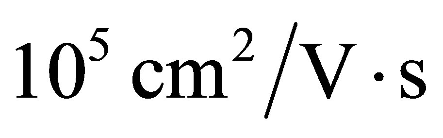 . Propagating ultrasonic waves can be amplified, depending on the electric field amplitude. Specifically, amplification occurs when drift velocity exceeds sound velocity. This scheme can be employed for efficient ultrasonic amplifier device operation.
1. Introduction
Ultrasonic waves are elastic waves consisting of frequencies greater than 20 kHz and exist in excess of Tera Hertz in graphene. Graphene utilizes ultrasonic waves in wide range of applications including acoustics, superconductivity and sensing. Ultrasonic velocity and attenuation are the important parameters required for ultrasonic technique of material characterization. The velocity is related to the elastic constants and density of material. Hence, information about mechanical, anisotropic and elastic properties of a medium can be determined from knowledge of the velocity change.
The discovery of graphene in 2004 sparked a wide range of research endeavors in this thinnest material. Despite its rich physics, there has been less exploration of acoustic characteristics of graphene. In sharp contrast, acoustoelectric properties of conventional two dimensional electron gas systems (2DEGs) has been greatly studied. Charge carriers in the 2DEG systems couples effectively with sound waves. Propagation and amplification of acoustic weaves in piezoelectric semiconductors was earlier studied theoretically in 1962 [1] and experimentally under crossed electric and magnetic fields [2]. We expect that, both the gapless and linear energy dispersion nature might allow graphene carriers to couple uniquely with sound waves.
At present, using semi-classical method to explore ultrasonic properties of graphene has not been studied greatly. However, a classical approach using nonlocal elasticity theory and incorporating small scale effects was employed to analyze ultrasonic wave propagation in graphene sheet [3]. We assume our graphene system is piezoelectric. This is quite good assumption, because acoustoelectric effect occurs in piezoelectric semiconductors with more than one carrier type, or in a multivalley band having well defined maxima and minima or a coaxed graphene consisting of holes with right geometry [4].
In this paper, we employ inverse piezoelectric effect to generate ultrasonic waves which interacts with massless Dirac fermions in graphene. We will consider, instead of just d.c field, a superimposed alternating field with frequency comparable to (or stronger than) the sound frequency. Considering a zero magnetic field, we will investigate frequency dependence of ultrasonic properties. Specifically, amplification characteristics of ultrasonic waves through attenuation and velocity change in graphene will be studied employing classical equations. It is often a good approximation to treat the problem of sound propagation in graphene as purely a mechanical problem once the influence of the relativistic 2D electrons is ignored.
2. Model and Propagation Equations
The model we considered here, which can easily be realized experimentally, is an engineered homogeneous piezoelectric Graphene Nanoribbon (GNR) or a graphene nanoribbon resting on piezoelectric substrate. A uniform applied time varying light beam
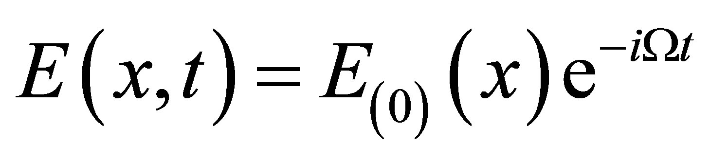 , (1)
, (1)
along the ribbon axis generates high frequency traveling acoustic waves within the medium. This effect is inverse-acoustoelectric effect. The direct effect will only be viewed as perturbations in the medium, as we will see shortly. In Equation (1),  is an a.c frequency and
  is static electric field amplitude. GNR is purely one-dimensional along propagation direction and has completely frozen out dynamics on the in-plane transverse and out-plain flexural modes. Actually, this makes our system slightly different from similar treatment using nonlocal elasticity theory [3,5,6].
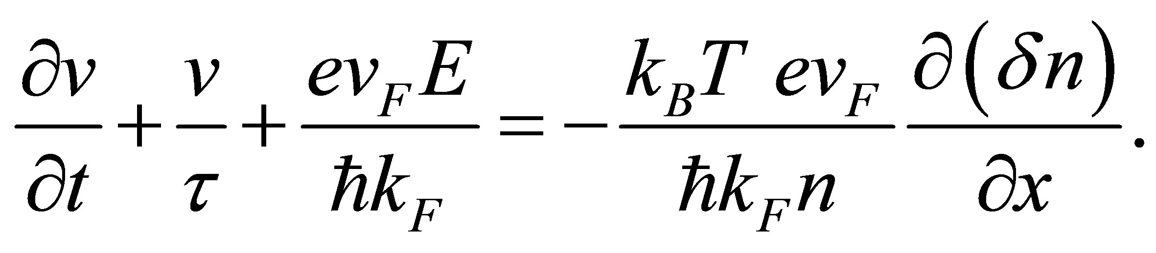
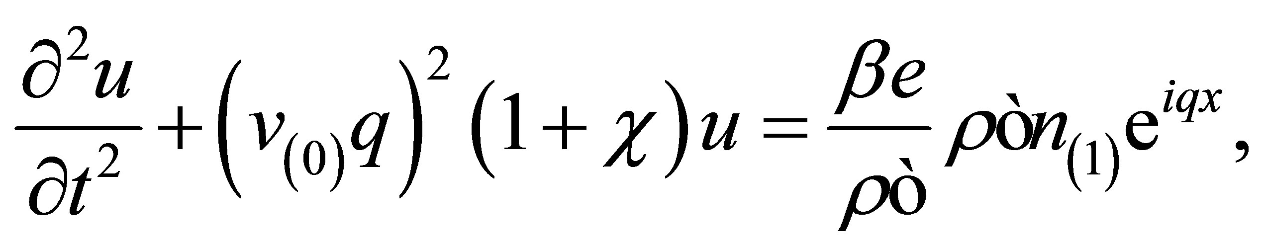
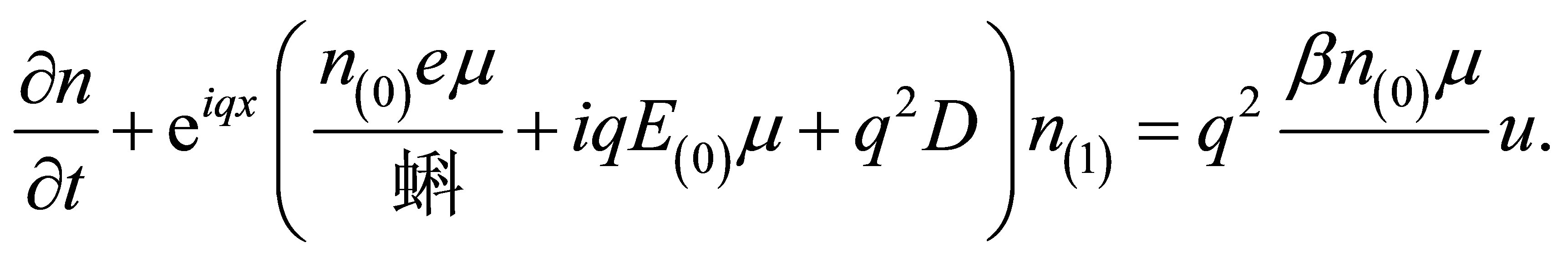
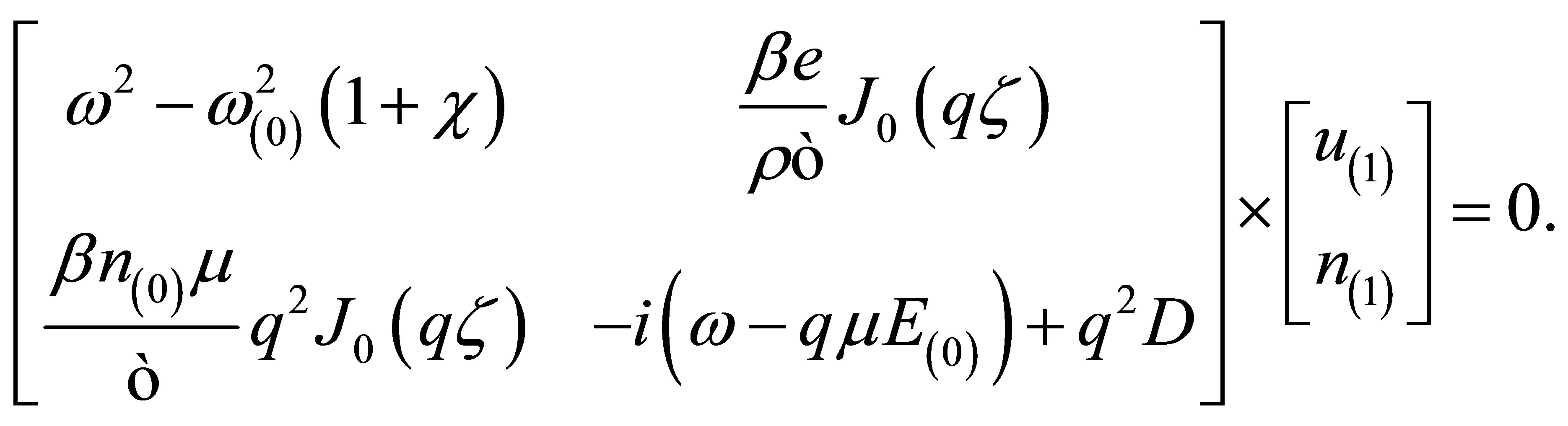
A system of coupled equations governing propagation of the generated acoustic waves, consists of Gauss, Poisson, and diffusion equations respectively;
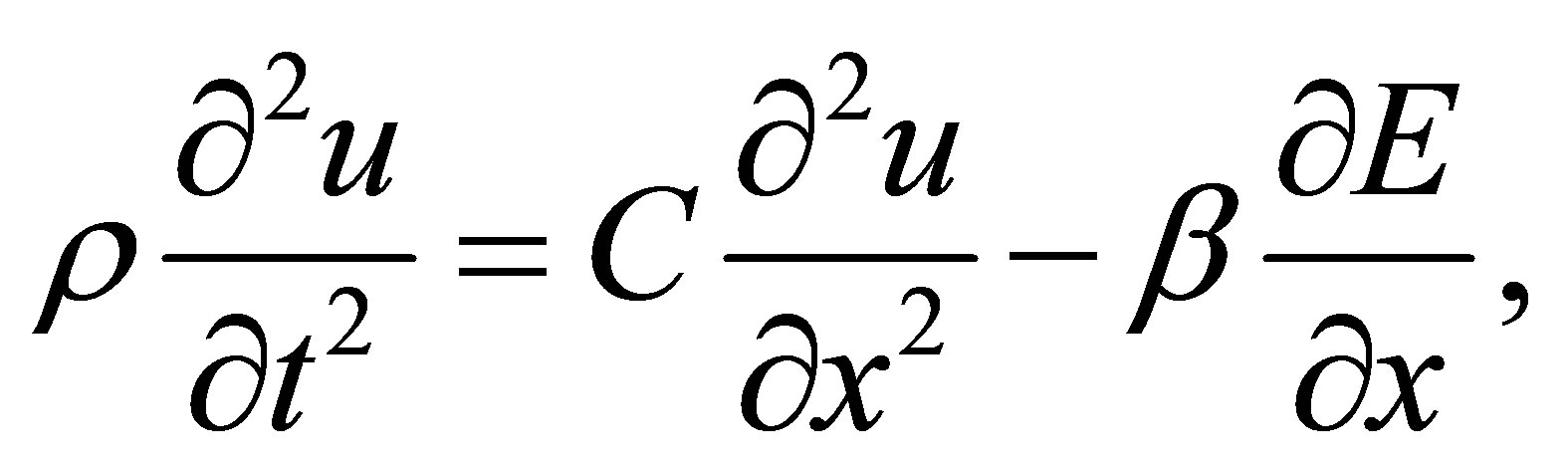 (2)
(2)
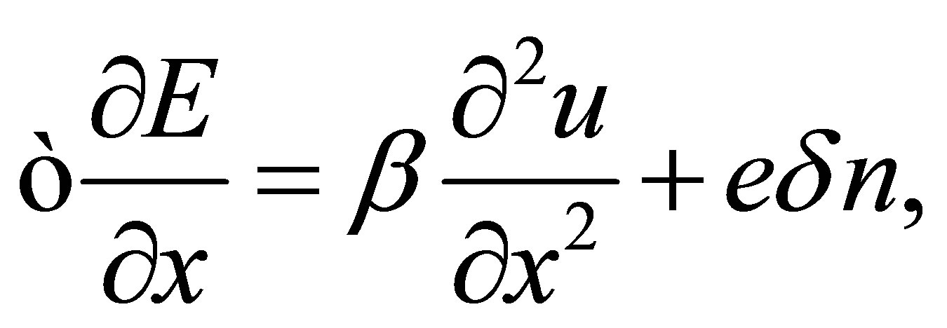 (3)
(3)
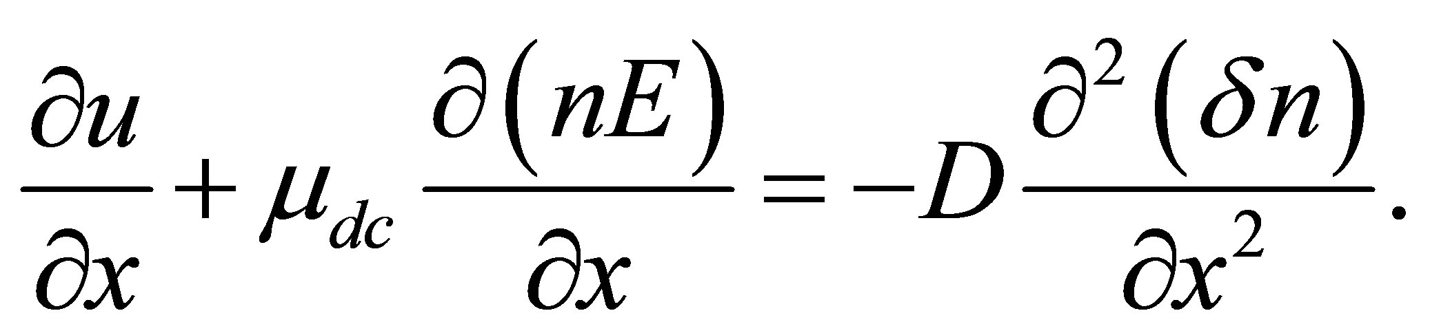 (4)
(4)
where  electronic density,
  piezoelectric coupling constant,
  dielectric permittivity,
  electric diffusion coefficient defined as
 ,
,  elastic modulation constant and
  electronic density fluctuation. An auxiliary equation for the velocity is also defined. i.e.,
 (5)
(5)
The differential Equations (2)-(5) are often solve to yield velocity change and attenuation of sound waves in a medium, if one considers two cases for the piezo-electric coupling; zero and finite coupling. In the following, we will show how these limits result in the solution.
2.1. Limit of Zero Coupling
For very weak or zero coupling of acoustic waves to the carriers, one can set . In addition, the absence of any source (such as gate voltage,
  often used in device applications) to control the electronic fluctuation means that
 . It turns out that, as in Equations (2) and (3), only plain wave solutions for
  are admitted and the electric field becomes constant,
 . However, a trial solution
 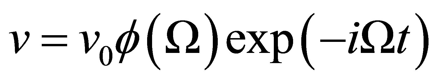 plugged in Equation (5) will produce carrier position with time
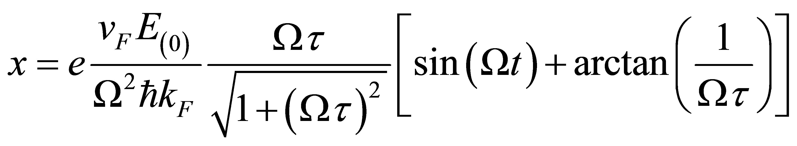 (6)
(6)
2.2. Finite Coupling
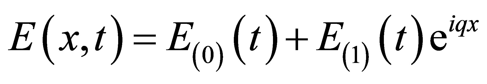
Now, for  sound waves couple effectively to dynamics of the carriers. The traveling ultrasonic waves caused by the external field produced perturbations on the system parameters. Specifically, a scalar potential induced is associated with an electric field
 , displacement vector,
 and number fluctuation,
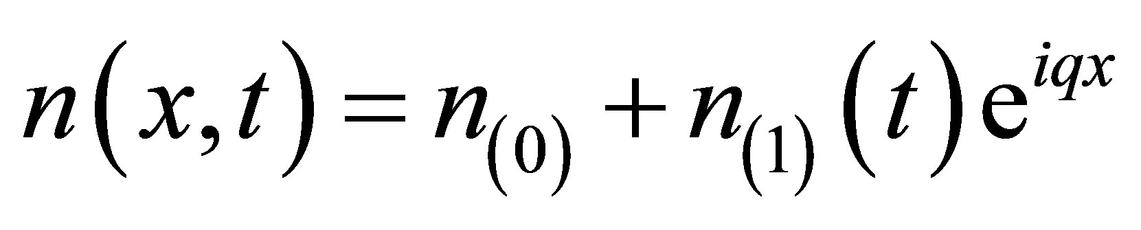
 . In view of these, we search for solutions with complex harmonic forms
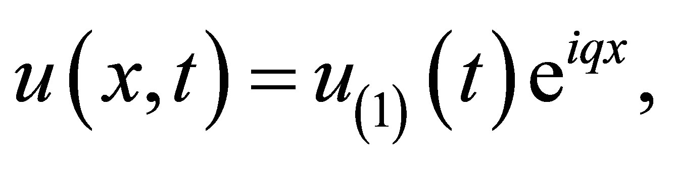 (7)
(7)
 , (8)
, (8)
 . (9)
. (9)
where  is the equilibrium number of electrons which produces electrical neutrality.
  is the deviation from equilibrium which has been defined as
 .
.  is the sinusoidal field amplitude due to the ultrasonic wave motion in the piezoelectric medium.
  is the induced displacement amplitude.
  is the wave vector along
 —direction. Substituting the harmonic solutions into Equations (2)-(5) immediately yields
 (10)
(10)
 (11)
(11)
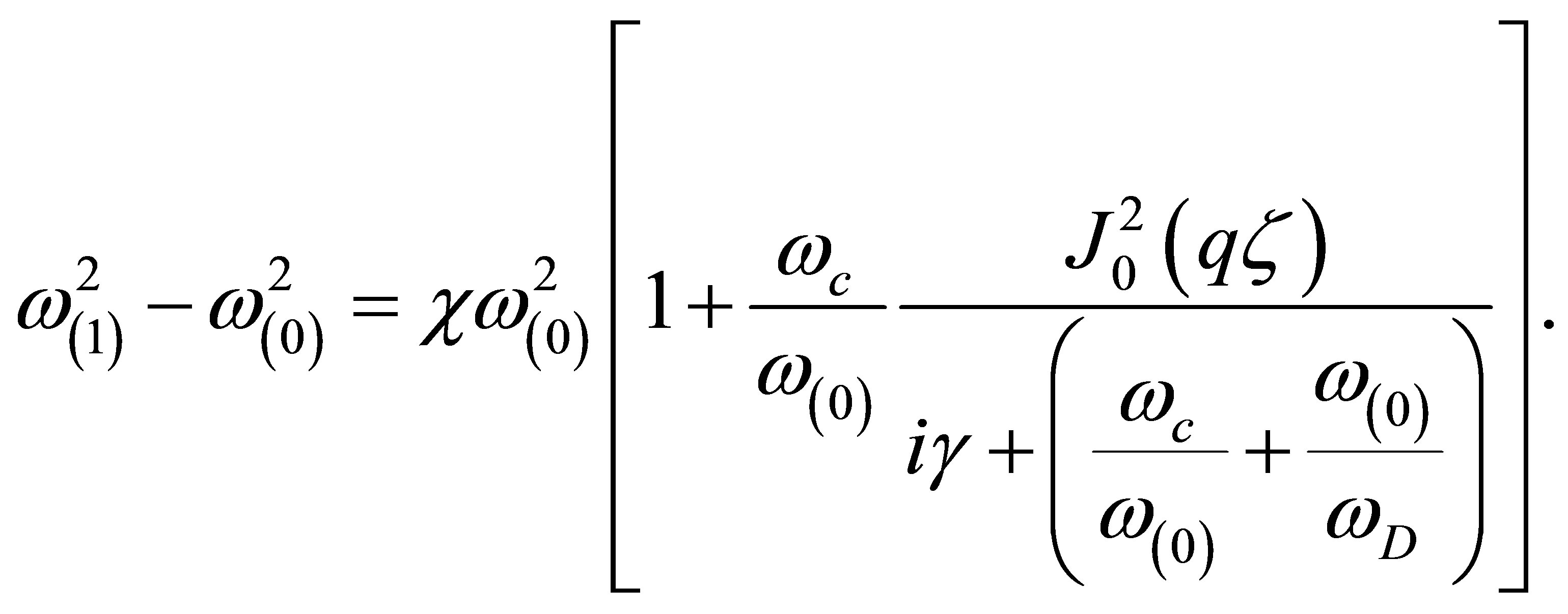
We have defined 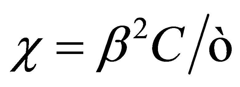 and
and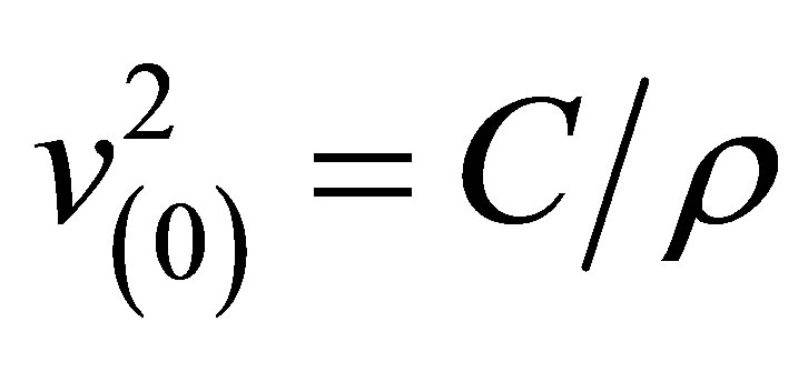 . Here, we do not make any distinction between longitudinal velocity,
  and surface Rayleigh waves,
 . In future, the product
  shall be replaced by unperturbed frequency
  Obtaining exact solution to these complex coupled Equations (10) and (11) is often difficult. Usually, the problem is well handled by adopting simplifying small signal approximations. For instance, the sound wavelength can be taken to be far longer than the electronic mean free path. Also, we assume a simple time dependence,
  for
for  and
and  It follows that,
 (12)
(12)
The Bessel functions,  are introduced through Jacobi-Anger expansions,
 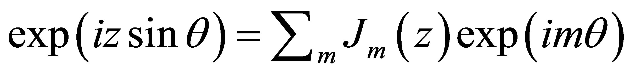 together with time averaging and retaining only
  order. In the argument of the Bessel function, zeta can be written as
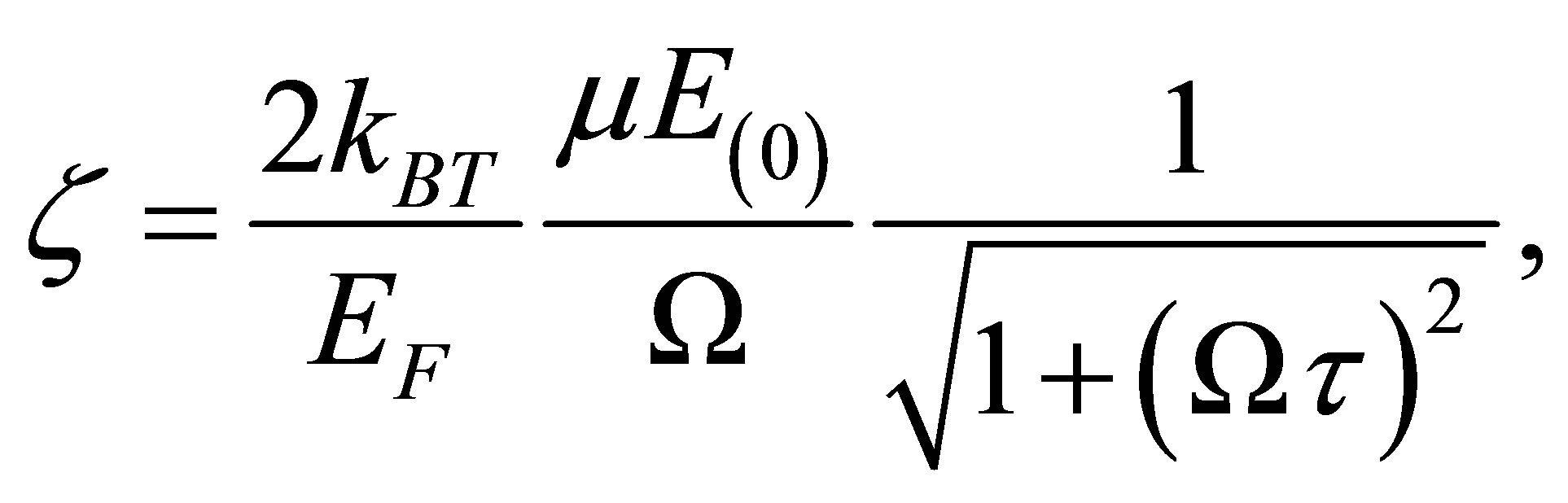 (13)
(13)
where we have used the relations  and
and . In the following, we defined system parameters such that
 is the dielectric relaxation frequency,
  is the diffusion frequency,
  is the drift frequency and
  is the normalized electric field (frequency). In Equation (12), we demand that
  so that a non-trivial frequency dispersion solution for the ultrasonic waves in terms of frequencies
 ,
,  and
and  becomes
 (14)
(14)
2.3. Iterative Solutions
In this section, we present approximate solution to Equation (13). The equation is complicated, since both sides contain . We seek an iterative solution by considering a situation where
 . Then,
 (15)
(15)
This is a zero order solution. It is very trivial and does not present any relevant physics. For second order iteration, the zero-th order approximation is substituted into the left hand side of the general solution to find
 (16)
(16)
Following this iterative procedure, and taking into account the fact that , the
, the  approximate solution takes the form
 (17)
(17)
It is immediately obvious from the preceding equation, that the presence of the complex term is an indication of wave attenuation in graphene.
3. Discussions and Conclusions
The velocity change and absorption of ultrasonic waves by Dirac fermions are defined as
 (18)
(18)
and
 (19)
(19)
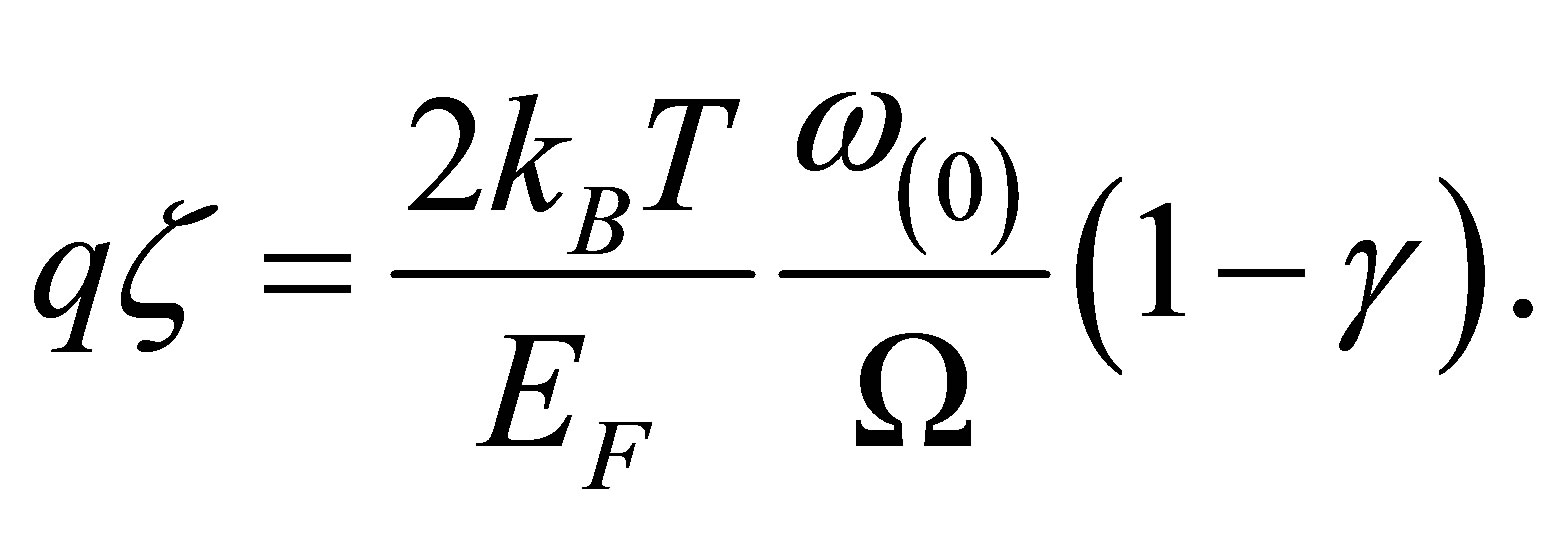
respectively. There are quite a number of system constants appearing in the ultrasonic physical observables of Equations (18) and (19). These must be fixed in order to proceed with any meaningful discussions. In the next section, we will attempt to estimate some of these parameters. Specifically, the electron mobility which fixes 
3.1. Numerical Estimates
In this section, we estimate electron mobility and the minimum electric field required to achieve the maximum reported electron mobility of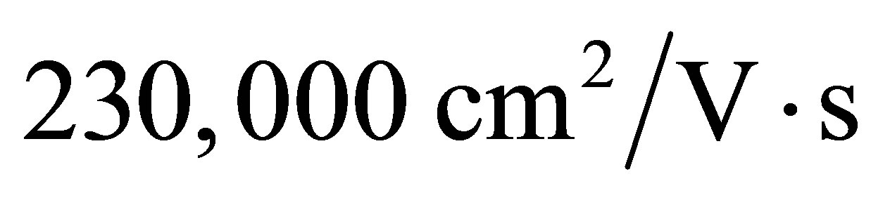 . In order to do this, it is appropriate that we fix the parameter
  that is valid for the conditions
 and
and  The Fermi energy
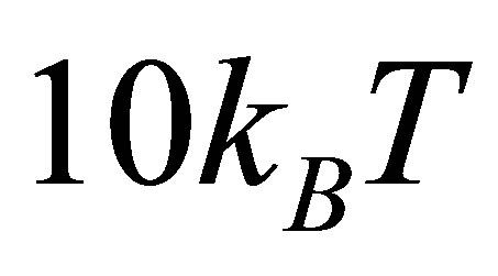 , so that thermal processes are minimal. In this limit, interactions of Dirac electrons with ultrasonic waves become an intra-band affair. Finally, we used
  as sound speed in graphene.
For time scales longer than the relaxation time,  (and for
 ), the argument of the Bessel function in Equation (13) modifies to
 (20)
(20)
We plot attenuation (absorption) with  and identified the roots as points of minimal or zero absorption of sound waves. A zero of Equation (19) is obtained at
 . This yields mobility of about
 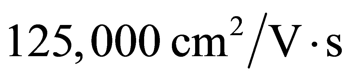 for
for . The numerical value has the same order as the one measured in [7]. The value can go higher for strong a.c frequencies, or for
  Since higher frequencies are possible in graphene as demonstrated in [8,9], where typical acoustic wave frequencies range from
 . The sensitivity of mobility to the electric field parameters indicates that
  can actually be tuned by those external factors,
  and
and 
3.2. Velocity and Attenuation Change with Frequency
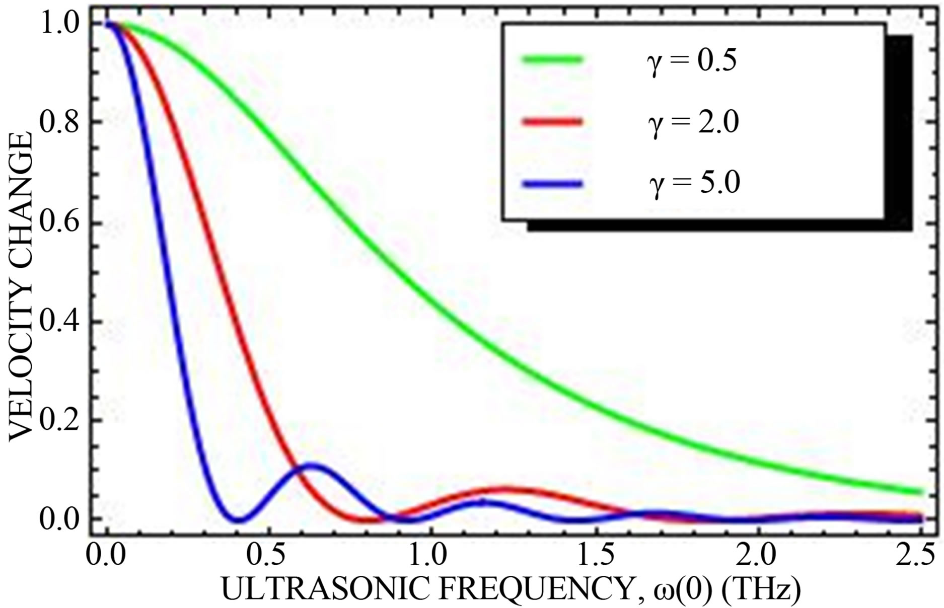
Here, we observe the behavior of physical observables as frequency and electric field amplitude are varied. Using Equations (18) and (19), we first plot velocity and attenuation with ultrasonic frequency in Figure 1. It is clear that at high frequencies velocity and attenuation disappears. Also, at small values of electric field amplitude, where , both observables are critically damped. However, as the drift frequency exceeds the sound frequency, i.e.
 , the curves quickly falls before beginning to oscillate at very low velocities where maximum absorption at low frequencies occur. The reason for these behaviors may be explain as follows; the high fields create electronic bunching which initially absorbed more of the sound and slows down the electron motion. However, over time there is debauching and the ultrasonic waves can now propagate in the system. The fact that graphene has unique energy spectrum may be responsible for the oscillations of the physical observables. This unusual feature is missing in conventional semiconductors [10] and two dimensional electron gas (2DEG) systems.
3.3. Amplification Scheme
Apart from the presence of complex term in the dispersion (19) which indicates a damped wave, there is also a possibility to get amplified waves depending on the value of . To get a feeling of the amplification, we plot absorption versus
  in Figure 2. The question now is how does one see amplification? In practical applications, amplification corresponds to negative attenuation. However, positive absorption will yield damping. From Figure 2, the region
  is where
  is negative. The ultrasonic waves are amplified in this region. Thus, the condition for amplification is
 . The equality holds at the beginning of the process.
4. Conclusion
We have studied ultrasonic properties of graphene sub-
 (a)
(a)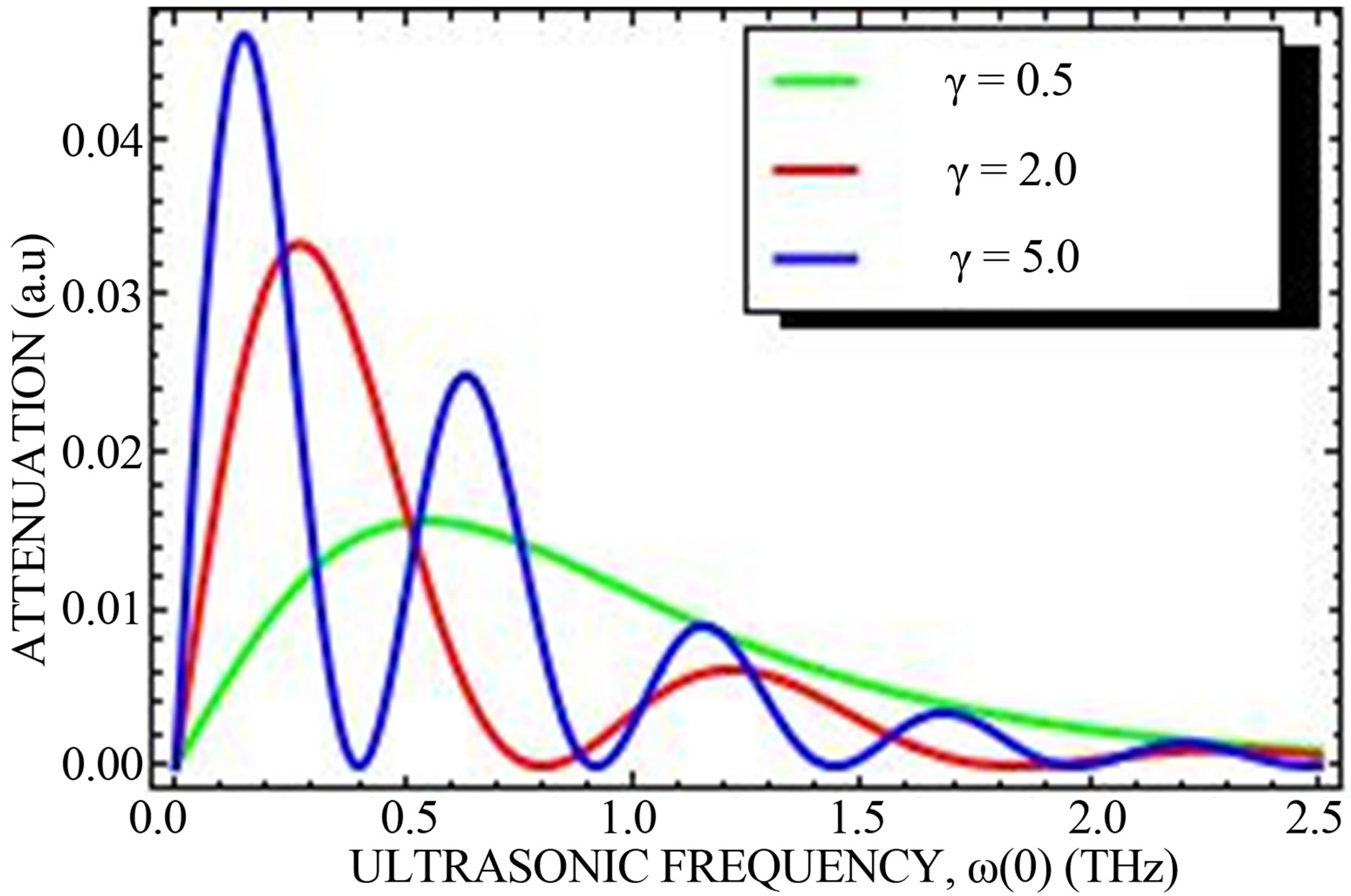 (b)
(b)
Figure 1. Behavior of ultrasonic physical observables with frequency.
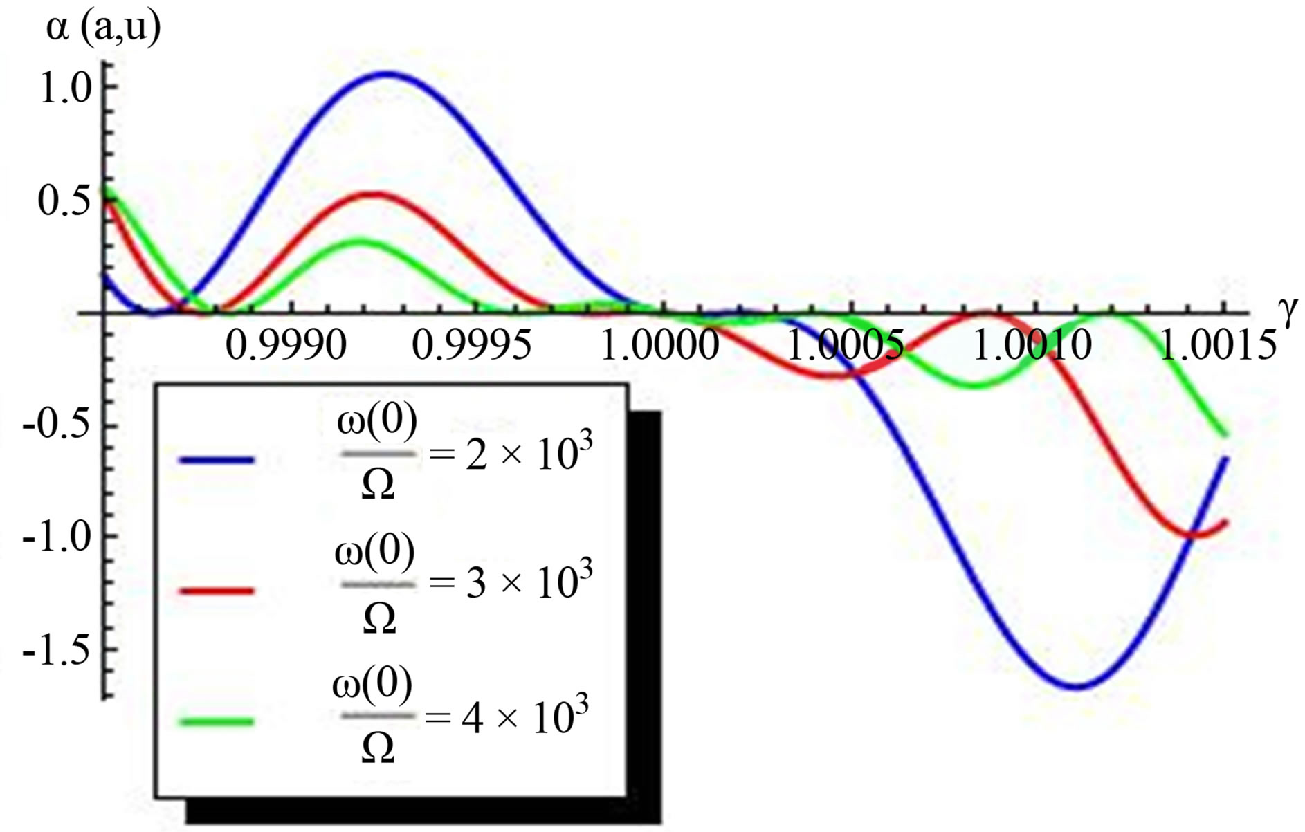
Figure 2. Amplification scheme for ultrasonic waves in grapheme.
ject to time varying external electric field. We observed unique oscillations of ultrasonic dispersion and absorption in contrast to conventional semiconductors that behave monotonically. This is due to the high fields creating electronic bunching which initially absorbed more of the sound energy produced and slows down the motion of Dirac electrons. However, debauching sets in after some time and the ultrasonic waves now propagate freely in the system. The unique electronic spectrum of graphene may account for such behaviors of the physical observables. We utilized the oscillatory nature of the absorption and velocity variation to compute electronic mobility which agrees quite well with reported values. The mobility can be tuned by the applied electric field amplitude. It is possible to have amplification of ultrasonic waves when drift velocity is larger than the sound velocity. An ultrasonic amplifier based on graphene devices and operating at higher frequencies can be very attractive.
REFERENCES
- D. L. White, “Amplification of Ultrasonic Waves in Piezoelectric Semiconductors,” Journal of Applied Physics, Vol. 33, No. 8, 1962, Article ID. 2547. doi:10.1063/1.1729015
- H. Hayakawa and M. Kikuchi, “Amplification of Ultrasonic waves under d.c. Operating Condition in InSb under Transverse Magnetic Field,” Applied Physics Letters, Vol. 12, No. 8, 1968, p. 251. doi:10.1063/1.1651978
- S. Narendar, D. Roy Mahapatra and S. Gopalakrishnan, “Ultrasonic Wave Characteristics of a Monolayer Graphene on Silicon Substrate,” Composite Structures, Vol. 93, 2011, pp. 1997-2009. doi:10.1016/j.compstruct.2011.02.023
- S. Chandratre and P. Sharma, “Coaxing Graphene to be Piezoelectric,” Applied Physics Letters Vol. 100, No. 2, 2012. Article ID: 023114. doi:10.1063/1.3676084
- B. Arash, Q. Wang and K. M. Liew, “Wave Propagation in Graphene Sheets with Nonlocal Elastic Theory via Finite Element Formulation,” Computer Methods in Applied Mechanics and Engineering, Vol. 1, 2012, No. 223-224, 2012, pp. 1-9.
- S. Narendar, D. Roy Mahapatra and S. Gopalakrishnan, “Investigation of the Effect of Nonlocal Scale on Ultrasonic Wave Dispersion Characteristics of a Monolayer Graphene,” Computational Materials Science, Vol. 49, No. 4, 2010, pp. 734-742. doi:10.1016/j.commatsci.2010.06.016
- K. I. Bolotin, K. J. Sikes, Z. Jiang, M. Klima, G. Fudenberg, J. Hone, P. Kim and H. L. Stormer, “Ultrahigh Electron Mobility in Suspended Graphene,” Solid State Communications, Vol. 146, No. 9-10, 2008, pp. 351-355. doi:10.1016/j.ssc.2008.02.024
- V. Miseikis, J. E. Cunningham, K. Saeed, R. O. Rorke, and A. G. Davies, “Acoustically Induced Current Flow in Graphene,” Applied Physics Letters, Vol. 100, No. 13, 2012, Article ID. 133105. doi:10.1063/1.3697403
- M. A. Paalanen, R. L. Willett, P. B. Littlewood, R. R. Ruel, K. W. West, L. N. Pfeiffer and D. J. Bishop, “Rf Conductivity of a Two-Dimensional Electron System at Small Landau-Level Filling Factors,” Physical Review B, Vol. 45, No. 9, 1992, pp. 11342-11345. doi:10.1103/PhysRevB.45.11342
- S. Y. Mensah, N. G. Mensah, V. W. Elloh, G. K. Banini, F. Sam and F. K. A. Allotey, “Propagation of Ultrasonic Waves in Bulk Gallium Nitride (GaN) Semiconductor in the Presence of High-Frequency Electric Field,” Physica E: Low-Dimensional Systems and Nanostructures, Vol. 28, No. 4, 2005 pp. 500-506. doi:10.1016/j.physe.2005.05.050