ABSTRACT

Theory predicts that the optimal foreign exchange rate policy of a central bank, in the presence of perfect capital mobility, and a persistent expansionary fiscal policy, is to fix this rate. Since these fundamentals apply to Lebanon, the Lebanese central bank has judiciously followed the policy of pegging the foreign exchange rate since the end of 1998. However, the actual policy led to a frantic quest for foreign exchange more than the level required or optimal. The behavioral model estimated in this paper worked endogenously from 1994 to 1998, and was actively operated upon afterwards. The model, based on financial engineering concepts, relates the change in the foreign exchange reserves of the central bank to the change in foreign exchange reserves of the banking system, and to the change in the foreign public debt. This model assumes that the central bank swaps government debt, denominated in Lebanese pounds, for a debt in foreign currency, thereby increasing its reserves, and improving the balance of payments. Moreover, the model is based upon the notion that the central bank is able to persuade banks to sell their excess foreign funds abroad for floating notes issued by the central bank, thereby increasing its reserves and improving the balance of payments. Although the central bank has announced publicly that it carried out the financial engineering embodied in the behavioral model discretely, and at specific periods, the paper finds that the same policy was continuously and incessantly undertaken and implemented, but at smaller scales. The crucial evidence comes about from the empirical finding that the change in the net foreign reserves of banks is positively, proportionately and significantly related to the central bank change in foreign exchange reserves. Moreover, part of the increase in foreign debt is funneled to a positive, and significant, relation with the change in foreign reserves of the central bank.

Keywords:

Central Bank, Foreign Exchange Reserves, Open Economy Macroeconomics, Foreign Exchange Rate Policy, Surplus in the Balance of Payments, Foreign Debt Policy, Financial Engineering, Lebanon

1. Introduction

One of the tenets of international finance is the “impossible trinity”. Domestic monetary policy cannot be independent in the presence of perfect capital mobility and fixed exchange rates, whereas fiscal policy is very effective and powerful in the same situation. This follows from the open economy IS/LM framework, as formulated by Mundell and Fleming, and which is still a paradigm in the international economics literature. See Fleming [1] [2] and Mundell [3] [4] . See also Daniels and VanHoose [5] .

An expansionary monetary policy will lead, at least in the short run, to a rise in aggregate output, coupled with a fall in the domestic interest rate. The fall in rates will induce a capital outflow which eliminates the fall and represents a deficit in the balance of payments. Foreign exchange reserves of the central bank will automatically be depleted, leading to a decrease in the monetary base, which results in a lower money supply. The ultimate contraction in the money supply totally reverses the initial expansionary policy, revealing policy incapacity.

Fiscal policy remains extremely effective. An expansionary fiscal policy will increase aggregate output, at least in the short run, and raise the interest rate. Capital mobility will ensure that a surplus in the balance of payments occurs, leading to more foreign exchange reserves of the central bank, higher monetary base, and more money supply. The latter in turn boosts aggregate output even further. However, in order to be effective, fiscal policy needs to be expansionary, and it needs to generate the cash flows necessary for the creation of a surplus in the balance of payments. Such a surplus is not evident because the public deficit that is required for an expansionary fiscal policy contributes to deterioration in international transactions, and may lead to a stagnant money supply, or even a decrease in the money supply. Therefore fiscal policy is effective only if it happens concomitantly with a surplus in the balance of payments. Of course, in the medium term, prices, which were assumed inflexible, begin to rise. A higher price level reduces the demand for real balances, and the LM curve shifts back to the initial position, i.e. before the fiscal shock. This effect is captured in the AS/AD (Aggregate Supply/Aggregate Demand) framework, which is considered to hold always (Challe, [6] ), or just in the medium run (Blanchard, [7] ). In fact the inflation rate did pick up later in Lebanon, and higher interest rates did edge upward. It seems that capital mobility was imperfect, and domestic interest rates were allowed to be higher than the world interest rate.

The governor of the Lebanese central bank was and still is hailed as immensely successful. By hindsight this was the consequence of a dual bet taken by the Governor of the central bank Riad Salameh. Part of his bet was to forecast that the future government stance, from the perspective of the mid 1990s and thereafter, will be mostly expansionary, in order to finance the destroyed infrastructure and rebuild the economic capacity of Lebanon. This bet was correct and Lebanese governments did pursue an aggressive fiscal policy, which fuelled the now elevated public debt. The second part of the bet was to forecast correctly that the balance of payments will remain in surplus. The remittances of the Lebanese, working outside, to the home country did not quench, and have been more than enough to finance the endemic current account deficit. This bet was that the Lebanese will continue their education, and become overqualified in their home country, thus increasing the domestic unemployment rate, necessitating their move to work outside in the rich Arab countries, from where they repatriated their excess funds to aid back their families.

Based on this dual bet the optimal monetary policy is to peg the foreign exchange rate. The bet turned out to be a winner, and the Lebanese pound stayed in the market within a narrow band from the end 1998s to the present. The byproduct of this bet was to enhance the banking system, helping it in attracting bank deposits and providing for earnings more than enough given the heightened financial activity. A negative byproduct is that the bulge in foreign reserves became associated with monetary stability. If foreign reserves increase the currency is seen as more and better backed up. However if foreign reserves decrease, after a shock, problems arise and the confidence in the currency is eroded. To prevent this erosion in confidence the central bank started to pursue frantic financial engineering operations to mitigate the shock to reserves. These operations consisted in a swap of Eurobonds with local currency debt, and encouraging financially banks to invest their foreign exchange reserves domestically. The first operation will boost the central bank’s foreign reserves because, upon its own admission, Eurobonds are considered to be part of its foreign and international reserves. The second operation, besides the increase in foreign exchange reserves, intended to refurbish the deficit in the balance of payments, and show decoratively a surplus, in order to appease the public sentiment. The new bet of the central bank is to maintain the accretion of foreign reserves at any expense, and to be correct on the forecast that the adverse shocks that Lebanon has faced or may face are and will be mainly transitory and temporary.

What is little known is that the central bank has pursued this financial engineering operation from the start, but, however, on a smaller scale. The main purpose of this paper is to explain the change in the central bank’s foreign reserves by relating this change to dollar repatriation of banks and to the change in the Eurobond public debt.

The initial impetus comes from the public which determines the assets in foreign currency of the banking system, and from the commitment of the central bank to follow a public debt policy. It will be shown that the change in foreign reserves of the central bank responds one to one to the change in the foreign reserves of the banking system that, in turn, is subjected to the desires and the decisions of the public in terms of dollarization. Hence an increase in the banks’ foreign reserves shows up as a decrease in the central bank’s foreign reserves. An increase in the latter comes about from the decrease in the former. There is weak evidence that the impact of changes of the foreign reserves of the banking system is more elastic for subtractions than for additions. The policy of the central bank of keeping a constant proportion of the public debt in its investment portfolio determines the residual part of the increase in the foreign reserves of the central bank. This means that the central bank’s policy of management of the foreign reserves is totally endogenous, reacting to the decisions of banks, originating from the public, and to the commitment of the central bank to hold a constant proportion of the foreign public debt, which stems from the government’s budget policy. The underlying thread is for the central bank to maximize as much as possible the level of foreign reserves, thereby showing external and internal strength, which is crucial in preserving the public’s confidence in the local currency especially in turbulent times. However, this has led to a frantic quest for reserves, which was made possible and was accommodated by the fundamentals.

This scenario has been pronounced in August 2016 and in May 2018. In August the banking system lost 2173 million US dollars which replenished the coffers of the central bank by part of 3939 million US dollars. In May 2018 the public debt decreased by 6594 billion of Lebanese pounds ($4396 million) which fed part of the 5133 million US dollars of the debt in Eurobonds.

The Lebanese central bank has the jurisdiction, the legalauthority, and the clear mandate to undertake these international transactions, in its pursuit of safeguarding the currency, maintaining economic stability, keeping an efficient banking system, and developing the monetary and financial markets. In addition the central bank is legally empowered to determine and modify the discount rate and its caps, and to purchase and sell bonds in the open market. This setup allowed the central bank to swap Treasury bonds in local currency held in its portfolio of securities to equivalent Eurobonds issued by the Treasury, and to sell dollar certificates of deposits (CDs) to the banking system, in return for their repatriation of dollar balances from abroad.

The expected impact of the financial engineering operations was to strengthen the foreign exchange reserves held by the central bank, while preserving exchange rate and interest rate stability, improving the balance of payments, and help in upgrading Lebanon’s credit rating.

The paper is organized as follows. Next, in Section 2, a brief literature survey on the accumulation of reserves is provided. In Section 3, the behavioral model is introduced and described. In Section 4 the empirical results are presented. Section 5 is a robustness check of these results. The last section summarizes and concludes.

2. A Brief Survey of the Literature

Before March 1973, central banks of countries that took part in the Bretton Woods meeting were obliged to hold foreign reserves, bearing in mind that they were committed to interfere in foreign currency markets, if their currencies’ rates were dragged out of a predetermined range. The breakdown of the system in 1973 was estimated to reduce central banks’ intervention in foreign currency markets, and therefore, reduce their demand for foreign reserves. However, central banks continued to maintain stockpiles of reserves, leading researchers to conclude that central banks have not altered their demand for foreign reserves with the change of the exchange rate system [8] [9] .

Batten [8] investigated the behavior of central banks regarding the demand for foreign exchange reserves within the framework of two models: the intervention model and the asset-choice model. The Intervention Model identifies four major determinants: 1) Variability of international payments and receipts, 2) Opportunity cost of holding reserves, 3) Scale variable measuring the size of international transactions, and 4) propensity to imports. In the Asset-Choice model, foreign reserves are treated as one type of asset in a central bank’s portfolio held to enable it to set up a local monetary policy.

The literature on reserve accumulation in developing countries, particularly in the Far East, is rich (see for example [10] [11] . Aizenman and Marion [10] examined why foreign reserves have been accumulated in the aftermath of the 1997 Asian crisis, in Asian countries, and what drives these accumulations.

Aizenman and Marion [10] set up a standard estimating equation, in which reserve holdings depend on scale factors, international transactions volatility, and openness, and effective exchange rates. They estimated reserve holdings to be positively correlated with the country’s population and standard of living, reserve holdings to be positively correlated with the volatility of a country’s export receipts, reserve holdings to be positively correlated with the average propensity to import, and reserve holdings to be positively correlated with exchange rate volatility.

Similar to [10] [11] found out that population and per capita GDP for economic size, ratio of imports to GDP, ratio of trade to GDP, and ratio of current account deficit to GDP for current account vulnerability, ratio of capital account deficit to GDP, ratio of short-term external debt to GDP, and ratio of broad money to GDP for capital account vulnerability, standard deviation of exchange rate for exchange rate flexibility, and interest rate differential for opportunity cost.

Gosselin and Parent [12] further examined the cointegrating vector by estimating a fixed-effects panel error-correction model for the percent change in the ratio of reserves to GDP, in order to evaluate the explanatory power of stationary variables that were initially dismissed from the cointegration analysis, like exchange rate volatility and opportunity cost.

The literature on the relationship between foreign exchange reserve accumulation and growth is also large [13] . Analyzing foreign exchange reserves as a percentage of GDP, Polterovich and Popovv [13] found that figures varied dramatically throughout the mentioned period, suggesting the lack of a relationship between foreign exchange reserves and GDP. Polterovich and Popovv [13] then examined the relationship between foreign exchange reserves accumulation and rates of long-term economic growth, assuming that there is a positive relationship between the two variables. Regression results showed that the investment/GDP ratios and growth are linked, but also suggested that reserve accumulation induce growth through greater involvement into foreign trade.

Bayat et al. [14] examined the asymmetric relationship between foreign exchange reserves and nominal―real exchange rate in the Turkish economy. However, they found that there is a causal relationship going from foreign exchange reserves to nominal and real exchange rates for raw data (positive relationship). There is a causality running from nominal exchange rates to foreign exchange reserves in the short run (a positive relationship also), and a causality running from real exchange rates to foreign exchange reserves in short and long run (again a positive relationship).

The literature on demand for foreign exchange reserves in Middle Eastern countries with a fixed exchange rate system includes a recent study on the relationship between foreign exchange reserves and the monetary base in Lebanon (Azar, [15] ). In his study, [15] also looked into the relationship between foreign exchange reserves and monetary base on one hand, and the broad money supply (M2) on the other hand, where the local currency is pegged to the US dollar. Azar [15] pointed out that in the long run, as the amount of foreign exchange reserves rises by 1 percent, the monetary base rises by one percent, regardless of whether foreign exchange reserves are valued in Lebanese pound or US dollars.

3. The Behavioral Model

The scenario is played by the public, the banking system, and the central bank. The public reveals its choice of dollarization, and its avowed desire to relocate savings back to Lebanon, or out of Lebanon. Banks decide to keep an optimal account balance in foreign exchange with foreign banks, especially with those that are correspondent banks. The central bank persuades the banking system to minimize these account balances abroad, and to redirect the funds back to Lebanon, and convinces them to swap long term denominated investments for a short run, and a higher floating rate investment at the central bank. The net effect is to show a balance of payments surplus on a net settlement basis, and a build-up of foreign reserves. Concomitantly the central bank agrees for another swap with the government, a swap of Lebanese-denominated debt for a Eurobond debt. These transactions with the government and the banking system result in a buildup in the portfolio of foreign reserves, granted that the central bank, by its own confession, considers Eurobonds as part of foreign reserves, and show a surplus in the balance of payments. Therefore it is with this gross amount of foreign assets and net surplus that the central bank publicizes its holdings of foreign reserves. The result is a frantic quest for foreign reserves, over and above what is optimal. More reserves serve to build the confidence of the public, which, in turn, give the public the incentives to repatriate its funds from abroad, and the cycle is chained together, in a virtuous circle. The unintended effect is that a fall in foreign reserves will break the cycle, and leads to a hysterical behavior of the public, leading the central bank to resort to this scheme as fast as possible.

The scenario was not ad hoc. It was planned since the early 1990s, but was only implemented in November 1998 by the celebrated peg of the Lebanese pound. Before this date the cycle fed itself endogenously, but, after that, it was a well guided policy. This is shown by the fact that the model for this scenario is estimated since January 1994, and the central bank had plenty of time, from then to November 1998, to learn the mechanism and act in due process. It is concluded that this scenario does not produce real changes in the structure of the economy, but is tantamount to be overt window-dressing.

To conclude the scenario and to construct the model, it is assumed herein that an increase in foreign reserves of the central bank comes about from two sources, one from the banking system, with its generation of a surplus in the balance of payments, and one from holding a certain proportion of the additional debt of the government in Eurobonds. The scenario, as will be shown, is not discrete, i.e. happening at a specific date, but continuous over the whole period. All this is well as long as the fundamentals espouse the virtuous cycle, or as long as the initial dual bet of the governor of the central bank perseveres and persists. However, beware of the down side…

Exhibit 1 portrays the evolution of the portfolio of the central bank in foreign reserves, without any gold valuation that was never traded, over the monthly period from January 1994 to August 2018. This graph shows the significant buildup in these reserves, especially since 2008. The graph can be considered also as a portrait of the frantic quest for reserves, or the enhanced appetite for reserves of the central bank during this current century. Statistically the geometric monthly growth rate is 1.132%, or 17.04% compounded annually. Compared to any scale of the economy of Lebanon this is definitely huge, and to say the least it is unwarranted.

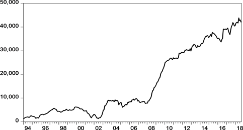
Exhibit 1. Total foreign exchange reserves of the central bank of Lebanon (in million of US dollars).

The second graph, Exhibit 2, shows the joint evolution of net changes in the foreign reserves of the central bank (in black), and the net changes of those of the banking system (in red). The negative relation is evident. The simple correlation coefficient is −0.69 that carries a t-statistic of −16.6904. This graph shows the extreme power of the central bank to convince banks to repatriate foreign currency and sell them to the central bank against the receipt of a floating-rate deposit still in US dollars. In other terms a deficit in the net changes of reserves of the banking system shows up as a surplus in the reserves of the central bank, creating a surplus in the official settlement balance of the balance of payments, and an increase in foreign reserves of the central bank

4. The Empirical Results

Based on the above, and adding the possibility of an asymmetric, non-linear, relation, the econometric model is as follows:

$\begin{array}{c}BDL={\beta }_1+{\beta }_{2}DUMMY\ast BANKS+{\beta }_3\left(1-DUMMY\right)\ast BANKS\\ +{\beta }_4\Delta \left(DEBT\right)+{\beta }_{5}AR\left(1\right)+\epsilon \end{array}$

In this equation BDL is the change is the foreign exchange reserves of the central bank (Banque du Liban), BANKS is the change in foreign exchange reserves of the Lebanese banking system, $\Delta \left(DEBT\right)$ is the change in the public debt in foreign currency of the Lebanese government, and DUMMY is an indicator variable that takes the value 1 if BANKS is negative, and zero otherwise. The variable $AR\left(1\right)$ stands for a first-order autoregressive process of the regression residuals. The coefficients ${\beta }_1,{\beta }_2,{\beta }_3,{\beta }_4$ and ${\beta }_5$ , are the regression parameters that are to be estimated. It is expected that ${\beta }_2$ and ${\beta }_3$ will be negative, and that ${\beta }_4$ is positive. The coefficient ${\beta }_5$ ought to be less than +1 to ensure stationarity and econometric stability.

Table 1 reproduces the results of putting to the test the above regression. Table 2 presents a list of hypothesis tests that are of concern. The statistical software used is EViews 10+ [16] . The method of estimation is ARMA Maximum Likelihood. Convergence is achieved after 10 iterations. The convergence tolerance is set at 0.0001.

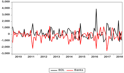
Exhibit 2. Changes in foreign exchange reserves (in US dollar million).

Sample: from January 1994 till August 2018. Sample size: 296 observations. Estimation is by ARMA Maximum Likelihood (OPG-BHHH). Convergence achieved after 10 iterations. Coefficient covariance computed using output product of gradients. Q(k) is the Ljung-Box Q-statistic of the residuals, for lag length k. Q² (k) is the Ljung-Box Q-statistic of the squared residuals, for lag length k. The normality test is the Jarque-Bera test. The Ramsey RESET test is carried out by including the square of the fitted value of the regression.

As expected ${\beta }_2$ and ${\beta }_3$ are negative. Banks sell their foreign exchange reserves to the central bank, and buy their foreign exchange reserves from the central bank. This leads to a 1 to −1 level relation. The estimates of ${\beta }_2$ and ${\beta }_3$ are close but less than −1. The coefficient on sales of reserves by banks is a bit higher in absolute values than the coefficient on purchases of reserves. The first is −0.800573, and the second is −0.638817. These coefficients are estimated with high precision. The statistical significance of these estimates is hence high. The t-statistics are respectively −18.24173 and −6.839123. However they are statistically significantly lower than 1, in absolute value. The respective two-sided actual p-values are 0.0000 and 0.0001.

These are impact effects. A long run effect can be found by multiplying ${\beta }_2$ and ${\beta }_3$ by $1/\left(1-{\beta }_5\right)$ , which is the long-run multiplier. This multiplier equals 1.331104, and is both statistically significantly different from zero, and statistically significantly higher than +1, and carry respectively actual two-sided p-values of 0.0000 and 0.0002. The multiplier shows that in the long run the impact is higher than in the short run, which is also as expected: adjustment takes time and is higher in the long run. The long run coefficients on banks sales and banks purchases of reserves are respectively −1.065645 and −0.850332. These two long run coefficients are statistically insignificantly different from −1. The actual two-sided p-values are respectively 0.4455 and 0.2605, failing to reject the null hypotheses of equality to −1. Finally both the two short run coefficients and the two long run coefficients are statistically equal, i.e. no different from each other. The actual two-sided p-values are respectively 0.1753 and 0.4021, failing to reject the two nulls of equality. Moreover these two long run coefficients are both no different statistically from −1 jointly. Hence there is no asymmetric effect and the relation is the same for purchases and sales of reserves. In many ways this is comforting, because it denotes that there are no privileges or hindrances attached to the side of the position in the foreign exchange transactions.

In Table 1, the change in the public debt in foreign currency, mainly in US dollars is positively related to the change in the foreign exchange flows. The coefficient on this variable is 0.165551, and carries at-statistic of 5.329664, making it highly significant statistically (the actual two-sided p-value is 0.0000). As expected this coefficient is between 0 and 1. Its interpretation is as follows: a one dollar increase in the public foreign debt is transmitted towards a 16.555% higher reserve position. In other terms, and on average, the central bank absorbs or holds 16.555% of the increase in the foreign public debt. The ultimate effect is an increase in the reserve position of the central bank, and a surplus in the Lebanese official settlement balance of the balance of payments.

The econometric diagnostics of the regression in Table 1 are not brilliant, except maybe for the R-square, and the Durbin-Watson statistic. Serial correlation of the residuals is present for lags higher than 3. Conditional heteroscedasticity for most lags fails to be rejected. The normality of the residuals is rejected at low marginal significance levels, and the Ramsey RESET test is negative. Granted that Ordinary Least Squares is usually robust to departures from the required assumptions, the Central Limit Theorem can be invoked to alleviate the effect of these departures, since the sample size is relatively large.

The results are subjected to many other hypothesis tests. The two first tests are whether ${\beta }_2-{\beta }_4=-1$ , and ${\beta }_3-{\beta }_4=-1$ , or whether the contribution to the reserves of the central bank are in totality one dollar for one dollar. The actual respective p-values are 0.5124, and 0.0464. Adopting a two-sided marginal confidence level and critical p-value of 1%, which is appropriate in finance research papers, the nulls cannot be rejected. In other terms there is no evidence that the sum of the total contribution is not unitary. The next tests are about the long run contribution:

$\frac{{\beta }_2-{\beta }_4}{1-{\beta }_5}=-1,\frac{{\beta }_2-{\beta }_4}{1-{\beta }_5}=-1$

The two tests find that the long run total contribution of sales of reserves by banks and for mopping up the foreign debt is statistically close to the adopted marginal significance level of 1%, and have respectively actual two-sided p-values of 0.0095, and 0.6319. Moreover the two long run coefficients of both sources of foreign reserves are jointly and statistically insignificantly different from −1, the actual p-value being 0.0338, which is above the cut-off rate of 1%, failing to reject the null of unitary long run impacts. Therefore the constraints hold and the following equalities also hold:

$\frac{{\beta }_2-{\beta }_4}{1-{\beta }_5}=\frac{{\beta }_3-{\beta }_4}{1-{\beta }_5}=-1$

The final set of results is about the autoregressive coefficient ${\beta }_5$. The implied long run multiplier is:

$1/\left(1-{\beta }_5\right)$

and carries a value of 1.33110, and a corresponding p-value of 0.0000, and is therefore highly significant statistically. In addition, and not only is it different from zero, but it is also statistically significantly different from +1, the actual p-value being 0.0002, rejecting the null of a unitary multiplier.

With the existence of an autoregressive variable the econometric model can be solved for the half-life of mean reversion, or sometimes called the median lag [17] . The original concept of half-life probably comes from the physical field. It measures the rate of decay of a particular substance. The half-life is the time taken by a given amount of the substance to decay to half its mass. Half-life gives the slowness of a mean-reversion process. It is equal to the following expression:

$\frac{\log \left(0.5\right)}{\log (\beta 5)}$

which is estimated to be 0.4982, and is highly statistically significant with an F-value of 47.48541 that carries a p-value of 0.0000. Since the data is monthly this estimate can be interpreted to be the time within which the long run is reached. This passage of time to the long run is indeed quite small, and is assessed to be around half a month. Therefore, the residuals of the econometric model above are relevant both in the short and in the long run, and are graphed in Exhibit 3 for the period after January 2010. Although the mean of this series is constructed to be zero, there is an indication that these residuals can reach either +1.6 billion US dollars and −1.2 billion of US dollars. These figures are astounding and may cast doubt on the model despite its high level of goodness of fit of 52%. However, the model should not be rejected for many reasons. First, there are lag/lead accounting adjustments in the residuals. For example, during

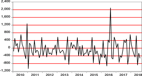
Exhibit 3. Net unexplained changes of the central bank’s foreign exchange reserves (US dollars million).

January 2011 an outflow of −1060.9 million US dollars was directly preceded by a cash inflow of +1268.9 million of US dollars during December 2010. Another example, a cash inflow of +2019.9 million US dollars during August 2016 was followed by cash outflows of −506.6 and −561.6 million US dollars during September and October 2016, respectively. Other examples can be found.

Another explanation, which is also in line with the model, is that these outlier gyrations are actually occurring in the population, being driven by a non-optimal management of exchange reserves. Knowing human behavior and despite the high competency level of policy makers, these extreme outcomes should not be surprising. Lastly, subjecting the data from January 2010 to August 2018, which is the period of Exhibit 3, to a normality test, provides for the results in Table 3. As can be seen from this table, and staying with the adopted marginal significance level of 1%, the null hypothesis of the normality of the residuals is not rejected. An additional piece of evidence, that supports the model, is the fact that the Chow breakpoint test produces very high p-values (0.9865), failing to reject the hypothesis of stability, when the selected break point is on December 1998, the date at which the central bank adopted a pegged foreign exchange rate. To conduct this test, the AR(1) variable must be replaced by the lagged dependent variable. The new model produces very similar outcomes as the AR(1) model, and will be rehearsed in the following section.

5. Robustness of Results

In order to check the robustness of the model, three alternative specifications are estimated (Table 4). The first replaces the residual autoregressive behavior with the inclusion of the lagged dependent variable. The second runs the regression with robust least squares, a method which adjusts for outliers in the dependent variable and in all independent variables. The third is a quantile regression evaluated at the median (LAD).

All coefficient estimates have the correct sign. These estimates are also close to each other. The estimate of ${\beta }_2$ varies between −0.684 and −0.801. The estimate of ${\beta }_3$ varies between −0.639 and −0.915. The estimate of ${\beta }_4$ varies between 0.0839 and 0.1656. The estimate of ${\beta }_5$ varies between 0.140 and 0.249. All coefficients are statistically significant, except for the estimate of ${\beta }_4$ in the quantile regression, which has, nonetheless the correct magnitudeand sign (0.119). The econometric diagnostics are similar. Higher order serial correlation of the

Sample: from January 1994 till August 2018. Sample size: 296 observations. Two-sided t-statistics are in parentheses. Two-tailed p-values are in brackets. Q (k) is the Ljung-Box Q-statistic of the residuals, for lag length k. Q² (k) is the Ljung-Box Q-statistic of the squared residuals, for lag length k. The normality test is the Jarque-Bera test. The Ramsey RESET test is carried out by including the square of the fitted value of the regression.

residuals fails to be rejected, while serial correlation is rejected for small lags. Conditional heteroscedasticity is not a major problem. Normality of the residuals is absent. The RESET test supports proper specification for the quantile regression, but not for the regression with the lagged dependent variable.

Whatever the econometric procedure the results are quite comparable, leading to the conclusion that, despite some statistical anomalies, the model is well framed, and is a good description of the posited behavioral model.

6. Conclusion

The central bank has judiciously followed a policy of pegging the foreign exchange rate. The policy is justified as long as there is a surplus in the official settlement balance of the balance of payments, and an aggressive expansionary fiscal policy. At least, this is what is predicted by the Mundell/Fleming IS/LM framework for the open economy. Although the theory is passé, it is nevertheless perfectly applicable to the state of affairs in Lebanon. The behavioral model estimated explains the changes in the foreign reserves of the central bank by those of the banking system, and by assuming a constant policy of absorption of the foreign public debt by the central bank. Although the model is small and structural it describes well what is anticipated from it, as exemplified by numerous hypothesis testing procedures. A danger zone is for the fundamentals to change, and necessitate official intervention on the foreign exchange market by the central bank, involving a sale of foreign securities to quell a possible devaluation. Another danger zone that comes about from the frantic quest for foreign reserves, is that a transitory shortfall of reserves will carry more meaning than it should, and thereby erode significantly more than it should the confidence in the Lebanese pound by the public. Such overreaction is not strange to financial markets, and is predictable in the field of behavioral finance [18] .

Conflicts of Interest

The authors declare no conflicts of interest regarding the publication of this paper.

Cite this paper

Azar, S.A. and Abdallah, H.J.K. (2019) What Drives the Accretion of the Foreign Exchange Reserves of the Lebanese Central Bank? (1994-2018). Theoretical Economics Letters, 9, 633-648. https://doi.org/10.4236/tel.2019.94043

References

- 1. Fleming, J.M. (1962) Domestic Financial Policies under Fixed and under Floating Exchange Rates. International Monetary Fund, 9, 369-379. https://doi.org/10.2307/3866091
- 2. Fleming, J.M. (1969) Domestic Financial Policies under Fixed and under Floating Exchange Rates. In: Cooper, R.N., Ed., International Finance, Penguin Books, New York.
- 3. Mundell, R.A. (1963) Capital Mobility and Stabilization Policy under Fixed and Flexible Exchange Rates. Canadian Journal of Economics and Political Science, 29, 475-485. https://doi.org/10.2307/139336
- 4. Mundell, R.A. (1968) International Economics. Macmillan, New York.
- 5. Daniels, J. and VanHoose, D. (2014) International Monetary and Financial Economics. Pearson, Boston.
- 6. Challe, é. (2016) Fluctuations et politiques macroéconomiques. Economica, Paris.
- 7. Blanchard, O. (2011) Macroeconomics. 5th Edition, Pearson, Boston.
- 8. Batten, D.S. (1982) Central Banks’ Demand for Foreign Reserves under Fixed and Floating Exchange Rates. Federal Reserve Bank of St. Louis Review.
- 9. Bastourre, D., Carrera, J. and Ibarlucia, J. (2009) What Is Driving Reserve Accumulation? A Dynamic Panel Data Approach. Review of International Economics, 17, 861-877.
- 10. Aizenman, J. and Marion, N. (2002) The High Demand for International Reserves in the Far East: What’s Going On? Working Paper 9266, National Bureau of Economic Research, Cambridge.
- 11. Prabheesh, K.P., Malathy, D. and Madhumathi, R. (2007) Demand for Foreign Exchange Reserves in India: A Co-Integration Approach.
- 12. Gosselin, M.A. and Parent, N. (2005) An Empirical Analysis of Foreign Exchange Reserves in Emerging Asia. Bank of Canada, Montreal.
- 13. Polterovich, V. and Popov, V. (2003) Accumulation of Foreign Exchange Reserves and Long Term Growth.
- 14. Bayat, T., Senturk, M. and Kayhan, S. (2014) Exchange Rates and Foreign Exchange Reserves in Turkey: Nonlinear and Frequency Domain Causality Approach. Theoretical & Applied Economics, 21, 27-42.
- 15. Azar, S.A. (2014) Foreign Reserve Accretion and Money Supply Creation: Lebanon’s Experience under an Adjustable Peg. International Journal of Financial Research, 5, 86.
- 16. (2017) EViews 10+. HIS Global Inc., Irvine.
- 17. Pindyck, R.S. and Rubinfeld, D.L. (1991) Econometric Models and Economic Forecasts. International Edition, McGraw Hill, New York.
- 18. Angner, E. (2016) A Course in Behavioral Economics. Second Edition, Palgrave Macmillan, London. https://doi.org/10.1007/978-1-137-51293-2