Theoretical Economics Letters
Vol.08 No.14(2018), Article ID:87895,34 pages
10.4236/tel.2018.814184
Innovation Clusters Effects on Adoption of a General Purpose Technology under Uncertainty
B. G. Jean Jacques Iritié
Department of Management, Business and Applied Economics, National Polytechnic Institute Houphouet Boigny, Yamoussoukro, Ivory Coast
![]()
Copyright © 2018 by author and Scientific Research Publishing Inc.
This work is licensed under the Creative Commons Attribution International License (CC BY 4.0).
http://creativecommons.org/licenses/by/4.0/


Received: June 30, 2018; Accepted: October 17, 2018; Published: October 20, 2018
ABSTRACT
This paper analyzes the effect of innovation clusters on the adoption of a general purpose technology (GPT) and on firms R&D investment levels in imperfect information situation. We developed a theoretical model of vertical relation, described as a four-step game between an upstream firm providing innovative GPT and an innovative downstream associated sector, integrator of this technology. The downstream sector ignores the quality of the GPT and we model the innovation cluster as a coordination mode of firms, improving the probability of the downstream firm to receive information about the quality of the GPT technology. Then, we determine firms equilibria (i.e. prices and technological qualities) and we showed that the effect of innovation clusters on the choice of qualities, the adoption behavior, levels of R&D investment as well as that social welfare depends on the quality of R&D activities carried out before the establishment of the clusters and a threshold effect (i.e. cluster critical mass); if the critical mass in terms of information sharing and interaction is not reached, the cluster may have negative effects. In other words, the consensual idea of expected positive effects of innovation clusters must be put into perspective.
Keywords:
Innovation Clusters, General Purpose Technology, Technological Complementarity, Technology Adoption, Uncertainty, Critical Mass

1. Introduction
Since the Silicon Valley success story in the US, innovation clusters are seen as central to innovation policy and economic development worldwide. In France, for example, the cluster policy concerns various technological domains and activity sectors. In this paper, we analyze theoretically the effect of the cluster policy on firms’ behavior in technology adoption as well as on firms’ R&D levels. To do this we will focus on nanotechnologies.
The nanotechnologies are currently qualified as general purpose technologies (GPT). The concept of GPT was introduced by [1] ; it refers to all technologies characterized by their strong technological opportunities1, their potential use as a factor of production in a large number of activity sectors, their technological dynamism and their technological complementarity with existing or potential technologies2. Bresnahan and Trajtenberg modelled a vertical relation between an upstream sector producing a GPT (semiconductor) and downstream user sectors (computers, hearing aids, TV, scanners); this supplier-customers relation is coordinated by market mechanisms without contractual relations between firms. The authors described it as a simultaneous game in which each sector chooses its level of R&D investment, thus evaluating incentives to innovate of firms. Bresnahan and Trajtenberg showed that incentives to innovate in the two sectors remain socially weak due to the presence of technological complementarity and vertical and horizontal externalities; these externalities raise coordination problems between innovation actors and give strong motivations to create and increase the degree of cooperation and contracts, on the one hand between GPT sector and associated sectors, and on the other hand between associated sectors. This result constitutes the starting point of our analysis. Indeed, for us, an innovation cluster can be considered as a response to the coordination problem between innovators highlighted by the authors; it is supposed to be a localized platform that allows increased information sharing and firms’ cooperation. As a result, the innovation cluster should play a facilitating role, the importance of which should be assessed in knowledge creation and technologies adoption.
The literature on adoption of new technologies is abundant. In a synthesis, [15] emphasizes two relevant characteristic features of theoretical models: the uncertainty and the strategic interaction in the final product market. As regards the first, several works such as [16] [17] and [18] show that uncertainty on profitability of new technology can reduce or increase incentive for adoption according to whether beliefs are pessimistic or optimistics; this points out the importance of gathering information3. The second element, i.e. the strategic interaction, implies that incentive to adopt for a firm depends on the adoption decision of rival firms4.
The model we develop is inspired, on the one hand, by the work of [1] and, on the other, by the theoretical work on the adoption of new technologies, notably the important contribution of [16] and its variants in [17] and [19] . Then, in order to analyze the impact of innovation clusters, we consider a vertical relation between a GPT supplier (upstream sector) and GPT integrators (downstream sectors); we suppose the vertical relation is coordinated either within an innovation cluster or by a classical market (i.e. outside the cluster). To capture the difference between the two coordination modes, it is assumed that their probabilities of receiving information about the upstream technology are different from each other. The vertical relation is described as a four-stage sequential game in which the downstream customer sector is confronted with the decision whether to adopt GPT innovation.
We solve the game and analyze the effect of innovation clusters on different equilibria. Our main results show that innovation clusters can positively or negatively influence the choice of qualities (i.e. technological levels), adoption behavior, upstream and downstream R&D investment levels as well as social welfare. However, this effect depends on the quality of the R&D activities carried out on the territory before the establishment of the cluster and on a threshold effect or cluster critical mass. If the critical mass is not reached, the innovation cluster can have negative effects. It can be deduced from this that the real issue for cluster policy is not only to increase the sharing of information and externalities of knowledge, but above all to allow this increase to be sufficient to reach a critical mass within the cluster; it is therefore necessary to put into perspective the expected positive effects of innovation clusters.
The rest of the paper is organized as follows. Section 2 presents the model. Sections 3 and 4 are devoted to the resolution of the game and to the determination of the equilibria of firms. We then analyze the effect of innovation clusters on the choice of upstream quality, on the downstream adoption behavior and on the social welfare in Section 5. In Section 6, we analyze an application with explicit functions. Finally Section 7 concludes the paper.
2. The Model
Setup. Let us consider the vertical relation between an upstream sector producing a good embodying a GPT and some downstream sectors, each developing an associated technology; there is technological complementarity between upstream technology and each downstream technology.
Let us suppose that the upstream sector is monopolized by a firm, called GPT-firm (indexed by g). In order to develop its technology with a quality z, (i.e. technological level), the GPT-firm invests in R&D, with and . To simplify matters, we assume that on the upstream market, the GPT’s firm may choose to produce low quality ( ) or high quality ( )5, its marginal cost of production is constant and given by c whatever quality z. GPT-firm sells its product to the user downstream sectors at a wholesale price w and realizes a net profit , being its gross income.
Now let us suppose a given downstream associated sector (AS)6 with a representative firm (indexed by a) of all downstream firms in this sector. The downstream firm carries out its own R&D program enabling it to develop a technology with quality k, , incorporated into a (semi-finished) product. The adoption of the GPT, combined with associated technology, allows the downstream firm to produce and sell a final good on the downstream market. The example of nanotechnology illustrates the technological complementarity in this vertical relationship7. Note that the downstream firm does not necessarily know GPT true quality because of imperfect information (or uncertainty); it only knows that z can take two values, or . It has however an a priori belief , , that the upstream GPT innovation is high quality ; is assumed to follow a distribution, is a probability density function.
Before deciding whether to adopt, the downstream firm receives or not information in form of a signal on the quality of the GPT; the signal arrives randomly with a probability h, ; once the signal arrived, it is perfect and reveals the true quality of the GPT. In other words, in the presence of the signal, the downstream firm is, ex post, in perfect information. In the model, we assume that the occurrence probability h of the signal depends on the coordination mode of the vertical relation; by this, we model the difference between two modes of coordination of innovation actors, i.e. the arm’s length market mechanism and the innovation clusters.
Let us suppose that on the market product of the downstream firm, all economic agents (downstream firm and customers) negotiate an efficient arrangement in order to maximize the gross surplus of the sector8. This assumes in particular that there is a monetary transfer from the customers to the downstream firm which ensures firm viability when gross profits do not cover fixed costs; our purpose here is to leave outside the scope of analysis all market imperfections. Thus, the gross surplus of the downstream sector is given by:
(1)
with the net consumer surplus, the unit production cost, the unit selling price of the downstream product; . To simplify notations, it will be assumed in the rest of the paper that without loss of generality. The demand of the GPT is given by with . We suppose that one unit of GPT’s good leads to one unit of the downstream good.
The definition of z and k implies derivatives and . We also suppose that , , , , , and . The hypothesis implies that the demand is decreasing with respect to . Otherwise, we note the R&D investment level, with , .
Timing of the game. We describe the vertical relation GPT and AS sectors as a four-stages sequential game:
- Stage 1 (R&D and upstream innovation). The upstream sector develops a product composed by GPT technology with quality , and choose a wholesale price .
- Stage 2 (signal on the quality). The associated sector receive or not information related to quality z as a signal; the signal is perfect and comes with a probability h depending on the coordination mode. In the presence of the signal, the downstream firm is in perfect information; but in the absence of the signal, it is in imperfect information.
- Stage 3 (adoption decision and downstream R&D). The downstream sector observes the GPT’s wholesale price and decides or not to adopt the GPT. If it adopts, it choose the level of its own associated technology and invests in research and development9. Then, it fixes its price .
- Stage 4 (revelation of z and downstream GPT demand). the quality z is revealed to all downstream sector’s agents (seller and final consumers); Consumers express their demands of downstream good; the AS-firm buys the necessary quantity of the GPT input and satisfies the demand of its product.
Remark 1. One can verify that even if the price pa is decided at stage 4, it would be the same as in stage 3; otherwise, we note that stage 4 suppose the GPT technology was adopted at stage 3.
We use backward induction to determine equilibrium of the game. First, we determine price and quality of the downstream sector in stage 3 for any value of w chosen by the upstream firm in stage 1 (we will deduce the demand and the profit in stage 4). Then, we determine the fist stage’s equilibrium of the upstream sector (expected demand, profit, quantity, price). Finally we proceed by static comparatives to analyse the effects of innovation clusters.
3. Downstream Firm Equilibrium
Perfect information. In the presence of the signal, the downstream firm observes the true quality of GPT. If it adopts technology, it chooses its technological level and fixes its optimal price which maximizes its profit . The choice of price is made by solving the maximizing problem of the downstream sector:
(2)
The first order condition leads to ; we verify that the price is given by:
(3)
The downstream sector’s gross surplus becomes and its net profit ; from assumptions on CS, we deduce the following properties: , , ; the inter-sectoral technological complementarity is given by .
The optimal quality k is given by:
(4)
respecting the first order condition [ ] and the second order condition [ ].
Note ; then the GPT of quality z is profitable (and will be adopted) iff 10.
Note that and respectively the optimal level of k and the associated maximum profit when the signal reveals and and the optimal level of k and the associated maximum profit when the signal reveals .
Remark 2. and are decreasing with respect to w.
Assumption 1. , and , .
By assuming and , we suppose there is always a price low enough for the downstream firm to be ready to adopt the low quality; for this low price, the downstream firm is ready to adopt even if it does not know the quality. In this case, the GPT is always profitable regardless the quality11. However, by assuming and , we suppose that for extremely high prices, adoption of GPT by downstream firm becomes unprofitable regardless of quality.
Lemma 1. There are two reserve prices, and , with and , such that: 1) the downstream firm adopts low-quality GPT technology iff , 2) the downstream firm adopts high-quality GPT technology iff .
We will see that ; in other words, in perfect information, the willingness to pay high quality ( ) is higher than the willingness to pay for low quality ( ).
Remark 3. We verify here the first part of the technological complementarity hypothesis highlighted by [1] . Indeed, we show that for all given w; in other words, in perfect information, the incentive to R&D in the downstream sector increases with the level of quality of the GPT technology.12
Proof. The first order condition implies ; which in turn implies that . By hypothesis and , thus .
We deduce the demand expressed by the downstream firm. It is a function of the both revealed quality z and wholesale price w of GPT good. Note that when the GPT good is of low quality and when it is of high quality; we distinguish the following three cases:
1) if then and the profit is given by while with a profit given by ;
2) if then and the profit is given by while and ;
3) if , the firm does not adopt whatever the quality of the GPT; and profits are zero.
Imperfect information. In absence of a signal, the associated firm is in imperfect information; it does not observe the quality z of the GPT. So, the firm’s adoption decision is based on its a priori belief that the technology is of high-quality. If it adopts, it choose its technology level and its optimal price so as to maximize its expected profit .
The choice of is solution of the maximizing problem of the firm’s expected gross profit:
(5)
with . The resolution
leads to a optimal price ; using this expression, the expected profit becomes .
The optimal k is given by:
(6)
Let us note . The GPT technology is profitable iff .
Definition 1. Let us consider as the reserve price of the downstream firm in the absence of the signal; then the firm adopts iff .
Lemma 2. is increasing with .
Proof. For any given w, . Let us suppose that for any firm i with an a priori belief , the GPT’s price is such as , then because is the price which cancels . Moreover by assumption, the profit of associated firms decreases with w. Consider a firm j with belief such as ; let us assess the firm j’s profit in ; we have
; the profit of firm j
assessed in is negative; knowing by hypothesis that the profit of j is decreasing with w and cancels in , it is therefore necessary to reduce to reach , which implies . Thus, we show that increases with ; in particular, .
Remark 4. In imperfect information, the reserve price depends on the a priori belief of the downstream firm. A very pessimistic downstream firm ( ) will have a stricter adoption criterion because its reserve price will be lower; on the contrary a very optimistic downstream firm ( ) will have a higher reserve price. Uncertainty can reduce or increase incentives for adoption depending on whether the firm’s beliefs are pessimistic or optimistic. The lack of signal can also lead to suboptimal behavior for the downstream firm; in fact, a pessimistic firm might refuse a high-quality GPT because the price w is such that , whereas in reality the firm would gain ex-post to adopt the GPT because it is of high quality . Similarly, an optimistic firm might adopt a low-quality GPT because the price w is such that while it would gain ex-post not to adopt the GPT because it is of low quality.
The purchasing behavior of the downstream firm in the absence of a signal depends on its reserve price, which is itself dependent on its a priori belief .
1) if , the downstream firm adopts the GPT; the anticipated demand13 on which it based its adoption decision at stage 3 is given by and its expected profit is given by ;
2) if , the downstream firm does not adopt the GPT; its anticipated demand is zero as well as its profit.
4. Upstream Firm Equilibrium
The expected demand of the upstream firm depends on available informations; let us note when the firm produces low quality and when it produces high quality.
Perfect information. In the presence of a signal, upstream and downstream firms have same informations; so the upstream expected demand is identical to the downstream firm demand in stage 4. Then,
1) if , we have and ;
2) if , and ;
3) if , ;
the corresponding profits are given by .
Imperfect information. In the absence of a signal, the expected demand of the upstream firm corresponds to the expectation of the downstream firm demand expressed in stage 4; indeed, at this stage, consumers observe the both GPT quality z and quality chosen by the θ-type downstream firm in the absence of signal. Then for an observed quality , we have and for an observed quality , we have ; therefore,
1) if , we have:
(7)
or
(8)
2) if , we have:
(9)
or
(10)
3) if , there is no technology adoption and the upstream expected demand is zero.
Imperfect information with signal probability h. If the GPT firm takes into account the probability h for the downstream firm to receive a signal on quality z of its product, its expected demand is a function of h. Indeed, GPT-firm knows that with probability h its expected demand is the same as in perfect information, and with a probability , its expected demand is the same as in imperfect information; so:
1) if , then
(11)
or
(12)
2) if
(13)
or
(14)
3) If the price of the GPT is such that , then the downstream firm does not adopt and the expected demand of GPT is zero.
Comparative static. Let us suppose that the downstream firm adopts GPT and let us analyze effects of the increase of h on the gap between the demand expected by the upstream firm when it produces high quality and the demand expected when it produces low quality, i.e. . To do this, let us consider two cases, either the upstream firm chooses a unique price regardless the GPT quality, either the upstream firm sets endogenous prices depending on the GPT quality:
1) the upstream firm sets a unique price for any given h; then expected demand gap14 according to values of are:
a) if , by using Equations (11) and (12), we have
(15)
b) if , by using Equations (13) and (14), we have
(16)
we know by assumptions that , and ; so the effect of h on the demand gap is positive, i.e. .
Let us calculate the profit gap, . The effect of h on the profit gap is given by ; the previous result on the demand gap induces .
These results show that when h increases, whatever the unique wholesale price , including the one that maximizes the profit of low quality , the gap of demand expectations of the upstream firm increases as well as profits gap; as a result, the incentive to sell high quality GPT rather than low quality GPT increases with the probability h of receiving the signal. The upstream firm can therefore always have an incentive to switch to high quality ; but this requires an increase in R&D costs, a wholesale price adjustment and a sufficient level of h so that the gross profit gap to be greater than the R&D cost gap.
2) the upstream firm sets endogenous prices according to the quality of GPT; so we will have .
Let us set respectively and the optimal price for high quality and low quality for a given h.
Assumption 2. Suppose, for any given h, .
With assumption 2, we assume that for a given value of h, the upstream firm sells the high quality at a price at least equal to that of the low quality. Let us assess the effect of a variation of h on the profit gap between high and low quality; using the envelope theorem, we show that the total differential of the profit gap is given by:
(17)
Proof.
(18)
By definition, , so Equation (18) becomes:
(19)
It’s the envelop theorem ; similarly, for the profit of low quality, we obtain:
(20)
Using Equations (19) and (20), we write the profit differential:
(21)
The sign of profit differential depends on signs of and .
Lemma 3. and .
Proof. It suffices to verify that with Equation (11) we have , with Equation (13) we have , with Equation (12) we have , and finally with Equation (14) we have . Using the initial hypothesis (i.e. increases with k) and knowing that , we can easily verify inequalities resulting from equations (11), (13) and (12); for the Equation (14), we also verify that because .
Remark 5. Lemma 3 implies but does not necessarily
implies when high quality and low quality are sold respectively at price and .
Lemma 4. ; i.e. the incentive of the GPT-firm to sell high
quality rather than low quality increases with the probability of receiving the signal.
Proof. Lemma 4 is the consequence of lemma 3.
5. Effects of Innovation Clusters
We assume that the probability of receiving the signal h depends on the coordination mode of the vertical relation between the upstream firm (GPT supplier) and the downstream firm (integrator of GPT). We model innovation clusters by an increase of h compared to the market mechanism; in other words, if and correspond respectively to the signal probability on the market and within the cluster, then . Indeed we assume that, in the presence of a innovation cluster, it is more likely for the downstream firm to receive information about the true quality of GPT technology than a firm on an arm’s length market; the economic literature on cluster policy argued that innovation clusters give an advantage to firms, not only in terms of transaction costs, but also in terms of sharing valuable information because of geographical proximity and localized knowledge externalities (see e.g. [24] [25] ). We will analyze innovation clusters effects on the choice of upstream quality and on the downstream adoption behavior of the GPT and on the social welfare.
5.1. Choice of Upstream Quality
We analyze here effects of an increase of h on the upstream firm behavior in its choice to produce high or low quality. The previous analysis of the profit gap with respect to h shows that this gap can become large enough for high values of h; in this case, the GPT firm would have to pay the extra R&D cost in order to produce high quality. On the other hand, the profit gap can sharply decrease for low values of h; the firm would then have an interest in favoring low quality. In particular, if h becomes zero, the GPT firm always chooses the low quality15 because of the strict increase of R&D costs, .
Assumption 3. Assume that, in perfect information, i.e. , the GPT firm always chooses the high quality .
Note that assumption 3 ensures that in perfect information, the R&D cost for high quality always remains reasonable so that the profit .
Proposition 1. There exists a limit value , such that if the GPT firm invests in low quality, if the GPT-firm invests in high quality.
Proof. Proposition 1 is the consequence of lemma 4 and assumption 3.
Corollary 1. If the increase of h allows to move from a to a , the innovation cluster switches the GPT firm from low quality to high quality.
5.2. Downstream Adoption Behavior
From the point of view of the upstream firm, the expected level of R&D investment and the expected level of use of the GPT product in downstream depend on h, i.e. the probability of observing the signal in downstream.
Let us consider a downstream firm with a given type ; note its expected level of R&D investment and its expected level of GPT product utilization16. We analyze below the effect of increasing of h, on and .
5.2.1. Investment Level in Downstream Quality
The expected quality of downstream technology is given by ; the total differential17 with respect to h is:
(22)
We distinguish here three effects of h on the expected quality of downstream technology:
1) is the direct effect of h
2) is the indirect effect of h through price.
3) is the indirect effect of h through change of upstream quality.
For this analysis of effects of an increase of h, one can distinguish two cases: the increase of h does not lead to a change in upstream quality, i.e. or ; and the increase of h causes a switch from low quality to high quality upstream, i.e. .
First case: the increase of h does not result in a change in upstream quality.
In this case, or . Note the expected downstream quality when the upstream quality is and when the upstream quality is ; we have:
(23)
(24)
Knowing that and , the overall effect of h on and on depend on the both effect of h on the upstream wholesale price and effect of the upstream wholesale price on the choice of associated quality in
downstream. If these effects are negligible, we have and ; in other words, the increase of h reinforces the downstream
R&D investment when the GPT technology is of high quality and lowers it when the GPT technology is of low quality. On the contrary, if these two effects are not
negligible, then the overall effect of h on depends on signs of , and , while the overall effect of h on depends on signs of , and .
Assumption 4. , and .
With assumption 4, we suppose that GPT firm raises its price with h when it chose to produce high quality and lowers its price with h when it chose to produce low quality. We suppose that the model fundamentals, i.e. functions of demand, cost, profit, surplus, ensure this assumption.
Given assumption 4, let us reassess the overall effect of h on and :
1) Overall effect of h on
- if and , we verify that the indirect effect through price is negative; so there is a reinforcement of the direct negative effect of h on .
- if and , we verify that the indirect effect through price is positive; which leads to a smaller decrease or an increase of as h increases.
2) Overall effect of h on
- if and , we verify that the indirect effect through price is positive; this reinforces the positive direct effect of h on .
- if and , we verify that the indirect effect through price is negative; this leads to a smaller increase or a decrease of with respect to h.
Second case: The increase of h results in a switch from low quality to high quality in upstream
Let us evaluate the sign of . We know that:
(25)
(26)
We can decompose and write:
(27)
If the effect of the upstream price on the downstream quality and the effect of h on the upstream price are negligible, then , , , with and , with . In this case, using Equations (25) and (26), we show that the two right-side terms of the Equation (27) are positive; indeed:
(28)
(29)
Thus, we show that ; the switch from low quality to high quality reinforces the cluster’s positive impact on R&D investments in downstream.
On the contrary, if the effect of the upstream price on the downstream quality and the effect of h on the upstream price are not negligible, we can assess the overall effect of h on the expected investment in downstream; by using assumption (4), we have:
- if and , we show that the first right-side terms of the
Equation (27), i.e. , has an indefinite sign whereas the second term, , is positive; we conclude that the sign of is indefinite. However, if the increase in upstream quality following the increase in the upstream price is very important, then we verify that .
Proof. See Appendix A
- if and , we show that the first right-side terms of the
Equation (27), , has an indefinite sign whereas the second term, , is negative. We conclude that the sign of is indefinite. However, if the decrease in upstream quality following the increase in the upstream price is very important, then we verify that .
Proof. See Appendix A
Proposition 2. If or or with , the
innovation cluster increases the expected investment in downstream quality when the GPT firm invests in high quality and lowers it when the GPT firm invests in low quality18.
Corollary 2. If the increase of h results in a switch from low quality to high quality in upstream, we have two cases: 1) if we neglect the effect of h on the upstream price and/or the effect of the upstream price on the downstream quality, then the innovation cluster’s positive effect on R&D investments in downstream is reinforced. 2) if we do not neglect the effect of h on the upstream price and/or the effect of the upstream price on the downstream quality, then the innovation cluster increases the downstream R&D investment iff the consecutive increase in the upstream price positively and strongly influences the choice of
downstream quality, i.e. and ; but the innovation cluster
reduces the downstream R&D investment iff the increase in the upstream price has a negative and strong influence on the choice of quality downstream, i.e.
and .
5.2.2. Level of Use of GPT Good in Downstream
The total differential of with respect to h is given by:
(30)
Equation (30) expresses four effects of variation of h on the deamnd of downstream firm:
1) is the direct effect of h on the demand.
2) is the indirect effect of h through price variation.
3) is the additional indirect effect of h through the variation of GPT quality.
4) is
the additional indirect effect of h through the variation of downstream product quality.
The first effect is interpreted as the observed upstream quality effect, the second as the price effect, the third as the upstream quality variation effect and the fourth as the downstream quality variation effect.
First case: the increase of h does not result in a change in upstream quality.
Let us note the expected quantity when the GPT quality is and 19 when the quality of GPT is . We have:
(31)
(32)
What is the overall effect of h on the adoption behavior of a downstream θ-type firm?
1) If the effect of the change in upstream price on the choice of downstream quality or the effect of the increase of h on the wholesale price is negligible, then only the direct effect and the indirect effect through price remain.
Remark 6. With assumption 4 and lemma 3, we verify that in the two demand cases and , the two remaining effects of h are opposite: 1) when the quality is high (Equation 31), the direct effect is positive whereas the indirect price effect is negative; 2) when the quality is low (Equation 32) the direct effect is negative whereas the indirect price effect is positive. The global direction of variation will therefore depends on the strongest effect; in other words, if in the both cases, the direct effect is stronger than the indirect effect, then overall increases with h while overall decreases with h.
In order to determine the global direction of variation of downstream demand with respect to h, let us evaluate and compare demands for extremes values of h, i.e. and , other things being equal.
Firstly, considering Equations (11) and (13); demands in stage 4 are:
(33)
(34)
We verify with assumption that and . We assume , which implies that .
Secondly, considering Equations (12) and (14), let us evaluate and compare demands for the extreme values of h, i.e. and . Let us begin with Equation (12).
(35)
(36)
We also verify with that and . With and assumption 4, we show that . This result is also verified for Equation (14) and in this case, .
2) If the effect of the change in the upstream price on the downstream quality is not negligible as well as the effect of h on the wholesale price, then given
assumption (4) and knowing that , the overall effect of h on the
expected level of use of GPT good in downstream depends on the effect of the wholesale price on the downstream technology quality.
Overall effect on :
- if and , then the additional indirect effect of h through
the variation of the downstream quality is negative, leading to a reinforcement of the negative direct effect.
- if and , then the additional indirect effect of h through
the variation of the downstream quality is positive, reinforcing the positive price effect. In total, there is a smaller decrease or an increase in the downstream level use of the GPT good when h increases.
Overall effect on :
- if and , then the additional indirect effect through the
variation of the downstream technology quality is positive; which reinforces the positive direct effect of h on .
- if and , the additional indirect effect through the variation
of the downstream quality is negative, reinforcing the (negative) indirect price effect. In total, we have a smaller increase or a decrease in the downstream level use of the GPT good when h increases.
Second case: The increase of h results in a switch from low quality to high quality in upstream
Let us calculate the sign of . We know that:
(37)
(38)
We can decompose and write
(39)
1) If we neglect the effect of the upstream price on the downstream quality and the effect of h on the upstream price and using Equations (37) and (38), we show that the first and the second right-side terms of Equation (39) are positive; in fact,
(40)
(41)
We have just shown that . Thus, by shifting the upstream firm from low quality to high quality, the innovation cluster improves further its positive effect on the downstream level of use of GPT product.
2) If we do not neglect the effect of the upstream price on downstream quality and the effect of h on the upstream price, then given assumption (4), let us calculate the overall effect of h on the expected level of use of the GPT product in downstream:
- if and , we show that the sign of the first right-side term
of Equation (39), , is indefinite while the second term, is positive; from this, we can deduce that the overall sign of is indefinite. However, we show that if the increase in downstream technology quality following the increase in the upstream price is very important, we have .
Proof. See Appendix B.
- if and , we show that the sign of the first right-side term
of Equation (39), , is indefinite while the second term, is negative. We conclude that the overall sign of is indefinite. However if the decrease of the downstream technology quality following the increase in the upstream price is very important, we have .
Proof. See Appendix B.
Proposition 3. If and are strictly monotonous with
respect to h, if or or with , then the
cluster policy increases the downstream expected level of use of the GPT good when it is high quality and lowers it when it is low quality20.
Corollary 3. If the increase of h results in a switch from low quality to high quality in upstream, we have:
1) if we neglect the effect of h on the upstream price and/or the effect of the upstream price on the downstream quality, the positive effect of the cluster on the level of use of the GPT good in downstream R&D is strengthened.
2) if we do not neglect the effect of h on the upstream price and/or the effect of the upstream price on the downstream quality, then the innovation cluster increases the expected level of use of GPT good in downstream iff the consecutive increase in the upstream price positively and strongly influences the
choice of downstream technology quality, i.e. and ; but the
innovation cluster lowers it iff this increase of upstream price negatively and
strongly influences the choice of downstream technology quality, i.e. and .
In sum, we note that Propositions 2 and 3 show that the positive effect of innovation clusters on the level of use of new technology and on the level of R&D investment in downstream is subject to conditions, in particular that the increase of h has no effect on the upstream price and/or that the effect of the increase of the upstream price on the downstream technology quality is either positive or negative but negligible.
5.3. Welfare Implications
We suppose for the social planner, initiator of the innovation cluster policy, that the social welfare is the sum of the expected surpluses of upstream and downstream sectors; it depends on h and on the quality of the GPT product observed by the downstream sector in stage 4. Let be this surplus; we note that because , , and .
(42)
Following the implementation of the innovation cluster policy, the increase of h induces a variation of the social welfare given by:
(43)
First case: the increase of h does not result in a change in upstream quality.
Let us note and the social surplus when final consumers observe low quality and high quality , respectively. The upstream profits and are known but the downstream profits and expected by the social planner are given by:
(44)
(45)
Remark 7. In the expression of downstream profits according to the social planner, we deliberately assume that the downstream sector always adopts, that is, ; in all other cases where it does not always adopt, analyses remain the same.
Let us determine the sign of and the sign of . We showed previously that and ; in other words, the information gain is beneficial to the upstream firm only when it produces high quality. Otherwise, we calculate:
(46)
(47)
In each of the two equations, there are three effects: the direct effect , the indirect effect through the variation of upstream price , and the indirect effect through the downstream quality .
We also assume that the profit of the downstream sector increases with the level of investment in downstream quality, that is to say that , , and .
1) If we neglects the effect of the change in the upstream price on the choice of the downstream quality or the effect of the variation h on the upstream wholesale price, then Equations (46) and (47) become respectively:
(48)
(49)
Using Equations (44) and (45), we show that:
(50)
(51)
By definition of and , we know that in Equation (50), is larger than and in Equation (51), is larger than , thus
showing that and . The information gain is always beneficial
to the downstream sector; indeed, this provides to the downstream sector to approach its optimal investment level and improve its profit by reducing either the risk of under-investment or the risk of over-investment due to imperfect information on GPT technology.
In sum, if we neglect the effect of h on the upstream price or the effect of the
upstream price on the downstream quality, then while the sign of his indefinite; in other words, the innovation cluster improves social
welfare and allows alignment of upstream and downstream sectors’ incentives when the GPT good is high quality. On the contrary, when the GPT good is low quality, the overall effect of the innovation cluster is ambiguous because the upstream and downstream incentives are not aligned.
2) If we do not neglect the effect of the change in the upstream price on the choice of downstream quality or the effect of a variation of h on the wholesale price, and given the assumption (4), we calculate:
Overall effect of h on and
- if and , then the price effect is positive and reinforces the direct effect while the indirect quality effect is negative, leading to a smaller increase or decrease of . However, if and , we will have ; we deduce that .
- if and , we have a positive quality effect as well as an positive price effect, reinforcing the direct effect. In sum . We deduce that the overall effect of the increase of h on is indefinite.
Overall effect of h on and
- if and , the quality effect is positive, reinforcing thus the positive direct effect while the indirect price effect is negative. So, we have a smaller increase or a decrease of . However if and , we have , involving .
- if and , the quality effect is negative as well as the price effect; there is therefore a smaller increase or a decrease in the downstream profit. However, if , , then . We deduce that the sign of is indefinite.
In sum, we showed that if the increasing of the upstream price significantly increases the downstream quality, the social surplus increases iff the upstream firm produces high quality.
Second case: The increase of h results in a switch from low quality to high quality in upstream.
Let us calculate , with .
We rewrite in the form:
(52)
In other words,
1) If we neglect the effect of the change in the upstream price on the choice of the downstream quality or the effect of the variation of h on the wholesale price, then the third right-hand term of Equation (52), that is to say , is positive, involving that .
2) If we do not neglect the effect of the change in upstream price on the choice of downstream quality or the effect of the variation of h on the wholesale price, and given Assumption 4 and the signs of in the previous section, we have:
• iff and , with and very large;
• indefinite sign, otherwise.
In sum, if we ignore the effect of h on the upstream price or the effect of the upstream price on downstream quality, the shift from low quality to high quality in upstream reinforces the positive effect of innovation cluster on the social welfare. On the contrary, if the effect of h on the upstream price or the effect of the upstream price on the downstream quality is not neglected, the switch to
high quality in upstream reinforces the positive effect of the cluster iff and , with and very large.
Proposition 4. If or or and with and very large, then the innovation cluster improves the
social welfare if and only if the GPT good is high quality and/or if there is switching from low quality to high quality in upstream.
In this section, we have developed and solved a model with general forms of demand and cost functions. The resolution is based on assumptions, in particular on equilibrium wholesale prices; now we must ensure that these assumptions are consistent with other assumptions of the model. In the next section, we use specific demand and cost functions and then, we verify these assumptions on equilibrium prices as well as the innovation cluster effects on the choice of GPT product in upstream, on the downstream adoption behavior and on the social welfare.
6. An Application
Let us suppose that the consumer surplus is given by with , and , thus implying that the consumer demand function is given by ; we verify assumptions ; ; ; ; ; ; ; ; .
Let us choose the R&D cost of the downstream firm; we also verify that and ; the cost function reflects a decreasing return of R&D investments. The objective function of the downstream sector, i.e. its total gross surplus, is given by:
6.1. Downstream Firm Equilibrium
Perfect information. In the presence of the signal, let us calculate the price, quality, profit and the demand expressed by the downstream sector at equilibrium.
The maximization of the gross surplus with respect to leads to the optimal price ; we rewrite and the profit is given by . We show that the level of quality k which maximizes the profit is given by with and . Note that here we can verify the technological complementarity, i.e. .
The maximum value of the profit is given by with and . We remark that , and ; that implies that the downstream firm always adopts whatever the price of GPT technology; in other words, .
From the above, it is possible to deduce the demand of the GPT good expressed by the downstream sector: and .
Imperfect information. In the absence of the signal, the downstream firm bases its decisions on its a priori belief that GPT technology is high quality. In order to choose its price, the firm maximizes its expected surplus . We verify that and the expected profit is given by . The level of quality k which maximizes this profit is given by . By replacing with its value in the expected profit function, we obtain the maximum value of the profit, .
We thus remark that and . We thus note that even in the absence of a signal, the downstream firm always adopts; therefore . In addition, the anticipated demand on which the downstream firm bases its decision to adopt at stage 3 is given by .
6.2. Upstream Firm Equilibrium
Perfect information. The demand expected by the upstream firm corresponds to the demand expressed by the downstream firm. When the upstream firm chooses low quality, we have with a profit ; on the contrary, when it chooses to produce high quality, and the associated profit is .
Imperfect information. The demand expressed at stage 4 by the θ-type downstream firm is either when it observes or when it observes . Knowing that and , we show that the upstream firm expected demands are:
(53)
(54)
The corresponding profits are and , respectively.
Imperfect information with signal probability h. The demand expected by the upstream firm is:
(55)
(56)
The associated profits are and , respectively. Let us note the price of low quality and the wholesale price of high quality. After calculations, we show that and
are identical and independent of h and constant: . Thus Equations (55) and (56) respectively become
and . The expressions of expected profits are and .
6.3. Effects of Innovation Clusters
Choice of upstream quality. It is easy to show that the gap of expected demand in upstream increases with h because and ; similarly, the expected profit gap of the upstream firm increases with h. Indeed, and ; thus we verify that the innovation cluster encourages the GPT firm to sell high quality rather than low quality.
Assuming that R&D costs in upstream ensure positive profits to the upstream firm, we can easily verify that there is a limit value beyond which the GPT firm switches from low quality to high quality . The innovation clusters therefore influence the choice of upstream quality.
Figure 1 illustrates this analysis.
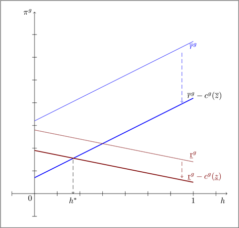
Figure 1. Profit gap.
Remark 8. We note that, for , iff . is solution of .
Downstream adoption behavior. Let us analyze the effect of the increase of h on the expected level of investment in downstream quality and on the expected level of use of the GPT product by a given θ-type downstream firm.
1) The expected qualities in downstream when the upstream firm produces low quality and high quality are respectively given by and ; once rewritten, we have and .
- If the increase of h does not produce a change in upstream quality, we show that and . In other words, the cluster encourages R&D investment in downstream when the GPT is high quality and discourages when the GPT is low quality.
- If the increase of h leads to a change from low quality to high quality in upstream, we calculate and we show that . Thus we thus verify that ; the shift from low quality to high quality reinforces the cluster’s positive impact on R&D investment in downstream.
2) The levels of expected use of the GPT good in downstream when it is high quality and low quality are respectively given by and .
- If the increase of h does not produce a change in upstream quality, we show that and ; the cluster thus increases the expected demand of GPT good when it is high quality and reduces it when it is low quality.
- If the increase of h leads to a change from low quality to high quality in upstream, we show that
; so we verify
that . The variation in quality, following the establishment of the cluster policy, reinforces the positive effect of the cluster on the expected demand for the GPT good in downstream.
Social welfare. Note respectively and the social surplus when consumers observe low quality and high quality . The upstream profits and are those calculated in imperfect information with signal probability h (see the previous Section 6.2). The downstream profits and are calculated according to Equations (44) and (45); we have:
We showed previously that and ; which means that the gain of information is beneficial to the upstream firm when it produces high quality. Moreover, after computation, we show that and , which verifies that the gain of information is always beneficial to the downstream sector. This allows it to move closer to the optimal investment level k, to improve its profitability by reducing the risk of under-investment or over-investment due to imperfect information.
Let us analyze the overall effect of the increase of h on the social surplus:
- If the increase of h does not result in a change in upstream quality, we immediately note that is positive. In other words, when the GPT good is high quality, the cluster system improves social welfare and facilitates the alignment of incentives of upstream and downstream sectors. On the contrary, the sign of is not immediate because incentives of upstream and downstream sectors are not aligned when the GPT good is low quality. Indeed, the calculation show that and then iff .
- If the increase of h causes a change from low quality to high quality in upstream, let us calculate the sign . We can decompose and write that ; we know that the first right-side term is positive. Let us develop the second right-side term like that: . We know that ; moreover, we verify with the equations of profits that , hence . In sum, we show that . In other words the shift from low quality to high quality in upstream, following the increase of h, reinforces the cluster’s positive impact on the social surplus.
Remark 9. We note that results in the above specific case are easy to read and
understand because we find , thus , and . Which shows that the upstream firm’s incentive to invest in R&D for
high quality comes from a volume effect and not from a price effect. In other words this comes from an exclusive effect of h on demand, i.e. a gain of additional information on the demand of GPT.
7. Concluding Remarks
This paper has focused on the theoretical analysis of the effects of innovation clusters on adoption behavior and the firms’ incentive to innovate in a vertical relation between a GPT provider and an associated innovative integrator. At the end of our analysis, we highlight three important results that need to be discussed; in general, these results show that the effect of the cluster depends on the quality of R&D activities carried out in the territory before the establishment of the cluster and a threshold effect or critical mass:
a) If R&D activities before the cluster are of low quality and the establishment of the cluster is sufficient to reach the threshold, then the cluster encourages the upstream firm to switch to a high quality technology. In this case, the upstream firm invests more in R&D; and as a result of the complementarity of technologies, the downstream firm is also encouraged to adopt and invest in high quality R&D; we show that social welfare increases.
b) If R&D activities before the cluster are of low quality and the establishment of the cluster does not achieve critical mass, then the cluster has no effect on quality. In this case, the innovation cluster has a negative effect (i.e. a disincentive) since the downstream firm will reduce its consumption of upstream technology; which will lead to a decline in upstream profit and social welfare.
c) If R&D activities before the cluster are of high quality, the cluster has no effect on quality; however, it encourages upstream and downstream firms to invest in R&D and the social welfare improves.
From these situations, we note it is in cases (a) and (c) that the establishment of the cluster generates the alignment of incentives (i.e. the best matching) of the upstream and downstream firms in terms of R&D, and leads to an improvement in social welfare. With regard to case (b), the establishment of the cluster leads to a disincentive and a decline in social welfare. In other words, the consensual idea of positive effects of clusters must be put into perspective.
It can be deduced from our results that the real issue for clusters is not only to increase information sharing; the increase should allow to achieve a sufficient level of information and interactions (i.e. critical mass) to encourage firms to conduct high-quality R&D. We can therefore safely maintain that there is no cluster if there is no critical mass. In fact, if there is not a critical mass of high-quality localized infrastructures, information and interactions, laboratories, firms in technologies and in given sectors, there will be no positive effects of innovation clusters.
Acknowledgements
This research was carried out during the author’s PhD research at University of Grenoble and Grenoble Applied Economics Laboratory (GAEL). It was supported by the PhD Scholarship Program Cluster 12 Region Rhone-Alpes―University of Grenoble (UPMF) FRANCE [Grant No. 348/PACT1-11111]. The author is indebted to the participants of SCSE (Mont-Tremblant Canada, 2012) and AFSE (Paris, 2012) annual conferences. We are also grateful to Eric Avenel, Christophe Bravard and Michel Trommetter for very useful comments on earlier versions of this paper. However the remaining deficiencies are the responsibilities of the author.
Conflicts of Interest
The authors declare no conflicts of interest regarding the publication of this paper.
Cite this paper
Iritié, B.G.J.J. (2018) Innovation Clusters Effects on Adoption of a General Purpose Technology under Uncertainty. Theoretical Economics Letters, 8, 2938-2971. https://doi.org/10.4236/tel.2018.814184
References
- 1. Bresnahan, T.F. and Trajtenberg, M. (1995) General Purpose Technology “Engines of Growth”? Journal of Econometrics, 65, 83-108. https://doi.org/10.1016/0304-4076(94)01598-T
- 2. Astebro, T.B. and Dahlin, K.B. (2005) Opportunity Knocks. Research Policy, 34, 1404-1418. https://doi.org/10.1016/j.respol.2005.06.003
- 3. Crampes, C. and Encaoua, D. (2005) Microéconomie de l’innovation, Editor: Economica, Encyclopédie de l’innovation, 405-430.
- 4. Youtie, J., Iacopetta, M. and Graham, S. (2005) Assessing the Nature of Nanotechnology: Can We Uncover an Emerging General Purpose Technology? Journal of Technological Transfer, 33, 315-329. https://doi.org/10.1007/s10961-007-9030-6
- 5. Menz, N. and Ott, I. (2011) On the Role of General Purpose Technologies within the Marshall-Jacobs Controversy: The Case of Nanotechnologies. KIT Working Paper Series Economics, 18.
- 6. Roco, M., Harthorn, B., Guston, D. and Shapira, P. (2010) Innovation and Responsible Governance. In: Roco, M., Mirkin, C. and Hersam, M., Eds., Nanotechnology Research Direction for Societal Needs in 2020, Springer, 440-487.
- 7. Graham, S. and Iacopetta, M. (2014) Nanotechnology and the Emergence of a General Purpose Technology. Annals of Economics and Statistics, 115/116, 5-35.
- 8. Thoma, G. (2009) Striving for a Large Market: Evidence from a General Purpose Technology in Action. Industrial and Corporate Change, 18, 107-138. https://doi.org/10.1093/icc/dtn050
- 9. Bozeman, B., Hardin, J. and Link, A.N. (2008) Barriers to the Diffusion of Nanotechnology. Economics of Innovation and New Technology, 17, 751-763. https://doi.org/10.1080/10438590701785819
- 10. Palmberg, C. and Nikulainen, T. (2006) Nanotechnology as a General Purpose Technology of the 21st Century? An Overview with Focus on Finland. DIME Working Paper Series.
- 11. Lipsey, R., Carlaw, K. and Bekar, C. (1998) The Consequences of Changes in GPTs. In: Helpman, E., Ed., General Purpose Technology and Economic Growth, MIT Press, Cambridge, 193-218.
- 12. Lipsey, R. and Carlaw, K. and Bekar, C. (1998) What requires explanation?. In General purpose technology and economic growth, Editors : Helpman, E. Cambridge: MIT Press, 14-54.
- 13. Jovanic, B. and Rousseau, P. and Bekar, C. (2005) General Purpose Technologies. In: Aghion, P. and Durlauf, S.N., Eds., Handbook of Economic Growth, Volume 1B, Elsevier B.V., 1181-1224. https://doi.org/10.1016/S1574-0684(05)01018-X
- 14. Jacobs, B. and Nahuis, R. (2002) A General Purpose Technology Explain the Solow Paradox and Wage Inequality. Economics Letters, 74, 243-250. https://doi.org/10.1016/S0165-1765(01)00551-1
- 15. Hoppe, H.C. (2002) The Timing of New Technology Adoption: Theoretical Models and Empirical Evidence. The Manchester School, 70, 56-76. https://doi.org/10.1111/1467-9957.00283
- 16. Jensen, R. (1982) Adoption and Diffusion of an Innovation of Uncertainty Profitability. Journal of Economic Theory, 27, 182-193. https://doi.org/10.1016/0022-0531(82)90021-7
- 17. McCardle, K.F. (1985) Information Acquisition and the Adoption of New Technology. Management Science, 31, 1372-1389. https://doi.org/10.1287/mnsc.31.11.1372
- 18. Reinganum, J.F. (1989) The Timing of Innovation: Research, Development and Diffusion. In: Richard, S. and Robert, W., Eds., Handbook of Industrial Organization, Elsevier B.V., 849-908. https://doi.org/10.1016/S1573-448X(89)01017-4
- 19. Jensen, R. (1988) Information Capacity and Innovation Adoption. International Journal of Industrial Organization, 6, 335-350. https://doi.org/10.1016/S0167-7187(88)80015-8
- 20. Mariotti, M. (1992) Unused Innovations. Bell Journal of Economics, 38, 367-371.
- 21. Kapur, S. (1995) Technological Diffusion with Social Learning. Journal of Industrial Economics, XLIII, 173-195. https://doi.org/10.2307/2950480
- 22. Reinganum, J.F. (1981) Market Structure and Diffusion of New Technology. Bell Journal of Economics, 12, 618-624. https://doi.org/10.2307/3003576
- 23. Karshenas, M. and Stoneman, P.L. (1993) Rank, Stock, Order and Epidemic Effects in the Diffusion of New Process Technologies: An Empirical Model. Rand Journal of Economics, 24, 503-528. https://doi.org/10.2307/2555742
- 24. Baptista, R. (1996) Research Round Up: Industrial Clusters and Technological Innovation. Business Strategy Review, 7, 59-64.
- 25. Stein, J.C. (1996) Conversations among Competitors. American Economic Review, 98, 2150-2162. https://doi.org/10.1257/aer.98.5.2150
Appendix A
Sign of when the increase of h results in a switch from low quality to high quality in upstream.
We know that:
- if and , we have:
In other words, the overall sign of is indeterminate.
However if and , then
possibly involving that ; we deduce that becomes overall positive.
- On other hand, if and , we have:
and the overall sign of is indeterminate. However if
and , then possibly involving
that ; we deduce that becomes overall positive.
Appendix B
Sign of when the increase of h results in a switch from low quality to high quality in upstream.
We know that:
- if and , and knowing that , we have:
The overall sign of is indeterminate. However if and , then possibly involving that ; we deduce that becomes overall positive.
- On other hand if and , we have:
The overall sign of is indeterminate. However if and , then possibly involving that ; we deduce that becomes overall negative.
NOTES
1In the French’s territorial configuration of clusters, nanotechnologies are developed within the cluster MINALOGIC (Grenoble, Region Rhone-Alpes). Let us note that the technological opportunities of a sector represent the potential for technical progress in the corresponding activity; then the notion of technological opportunity refers, for example, to the fact that 1 Euro invested in research does not necessarily leads to the same gain of productivity according to the technological potential of the activity in which it is invested [2] [3] . [4] give an interesting discussion about the nature of nanotechnologies. For further reading and discussions, refer to [5] - [12] .
2Following [1] , other works have focused on the analysis of the characteristics of GPTs; [12] explains that GPTs involve both enormous technological and Hicksian complementarities, [11] and [13] emphasize the relevant changes brought about by the discovery of a GPT (e.g, structural changes, public policy changes, etc.), the transient decline in productivity at the macroeconomic level generally observed after the introduction of a GPT, called the “Solow Productivity Paradox” (see also [14] ).
3For example, the gathering of information by observing the experience of first adopters is named social learning in [20] and [21] ; these authors showed that the social learning perspective delays adoption, except in the presence of explicit coordination of adopters.
4 [22] and [23] argued that rivalry can therefore accelerate adoption or delay it according to the advantage of the firm.
5This assumption makes abusive all derivation notations with respect to z; but we maintain them to recall the general case.
6As mentioned in the introduction, a general purpose technology (GPT) is used in several application sectors. However, if we consider that these application sectors (AS) are not necessarily interconnected and are independent of each other, they can be analyzed separately. Because of that, we do not model the horizontal externalities that could possibly exist.
7Indeed, many research programs are currently being undertaken in the field of microprocessors composed of integrated circuits on the molecular or nano-metric scale by exploiting the properties of individual silicon atoms. If they are actually produced and marketed, the use of these next-generation processors by computer manufacturers could enable to manufacture computers with ultra-low power consumption. In this example, the GPT product is the microprocessor integrating nanotechnology whose quality z would be measured by its ability to lower energy consumption; the downstream semi-finished good would be all the technological environment of the computer (CPU and everything in it) without the microprocessor; the technological level of this environment is given by k. The performance of the final good (i.e. the complete computer) will therefore depends on the associated technological levels k and z.
8Hence, in the rest of the paper, when we write gross profit (or respectively net profit) of the downstream firm, it is actually the gross profit (or respectively net profit) of surplus of the downstream sector.
9There is an offset between stage 3 and stage 4 because R&D requires time.
10If , the downstream sector does not adopt the GPT and chooses an opportunity action. We will normalize the opportunity cost to zero if technology z is an essential input; contrariwise if z is not an essential input, the downstream sector use an alternative technology.
11It is quite possible to assume that , which means that the adoption of GPT is profitable to the downstream firm if the quality is high ( ) and unprofitable if the quality is low ( ). [16] adopted this posture in its pioneering model of adoption and diffusion, a model generalized by [17] .
12In our model and at this stage, we assume that the choice of z and w is exogenous. In their article, [1] also model the choice of the GPT’s sector and show that the technological level of the GPT increases with k through the demand , i.e. . The technological levels are thus characterized as strategic complements.
13Indeed, in imperfect information situation, the expected surplus is given by , hence .
14To simplify notations, we write and .
15In the absence of a signal, the GPT firm has no interest to choose the high quality because the downstream sector ignores the quality. If the GPT firm chooses high quality, it invests more fixed cost in R&D while it receives the same demand and income as low quality. However, in a dynamic model integrating reputational aspects, one could imagine that the GPT firm chooses the high quality in the absence of signal to build or preserve its reputation.
16We note that and , because variables , , and are endogenous.
17Let us recall that because the variable z takes only two values, notations , and are abusive.
18In Proposition 2, k represents the both and and represents when GPT firm invests in high quality. Alternatively, when GPT firm invests in low quality, then k represents the both and and represents .
19We note that and for a given θ-type firm.
20In Proposition 3, k represents the both and and represents when the GPT-firm invests in high quality. Alternatively k represents the both and and represents when the GPT-firm investsin low quality.