Theoretical Economics Letters
Vol.4 No.3(2014), Article ID:44803,11 pages DOI:10.4236/tel.2014.43030
Land Productivity Changes in a Trade Liberalization Environment: Mexico under NAFTA
Diego de la Fuente Stevens1,2
1Former Address: Instituto Tecnológico Autónomo de México (ITAM), México City, México
2Current Address: Universidad Nacional Autónoma de México (UNAM), México City, México
Email: ddelafs@unam.mx
Copyright © 2014 by author and Scientific Research Publishing Inc.
This work is licensed under the Creative Commons Attribution International License (CC BY).
http://creativecommons.org/licenses/by/4.0/


Received 16 October 2013; revised 16 November 2013; accepted 30 November 2013
ABSTRACT
The focus of this research is the understanding of a fundamental aspect of the Mexican agricultural sector: the evolution of land productivity and the sources behind its changes. The study takes place in a period that runs from 1990 to 2011, a period of large structural transformations in the Mexican economy. The research offers answers regarding how the sector has adapted in terms of crop selection. Results show that a large share of total agricultural land productivity changes happened due to intrinsic changes in crop productivity; while these changes have different sources, most of them were the result of changes in production patters across states. Furthermore, around one quarter of total productivity, changes resulted from a better selection of crops in terms of productivity levels.
Keywords:Latin America, Mexico, Agriculture, Productivity, NAFTA

1. Introduction
During the second half of the 1980s and early 1990s, the Mexican economy experienced a series of structural changes that had an impact on the agricultural sector. After decades of trade protectionist policies, the country pursued an aggressive process of trade liberalization and in 1994 Mexico becomes part of a commercial integrated region with the signing of the North American Free Trade Agreement (NAFTA) with Canada and The United States. This treaty covered the gradual but continuous liberalization of the agricultural sector, something that had been missing on other trade reforms.
The changes in policy were partly devoted to bringing macroeconomic stability to the Mexican economy and partly the result of a search for industrial development that was supposed to be followed by rapid growth. It partially brought stability and industrial development but did not bring economic growth, see Tornell, Westermann, Martinez [1] , Hanson [2] and Kehoe and Ruhl [3] . Furthermore, the process of industrialization in the cities came accompanied with high internal migration, from rural to urban areas, see Levy and van Wijnbergen [4] , probably as a result of what Lewis [5] and Ray [6] explain as a complementarity between sectors that generates flow resources, in the form of labour, from the agricultural sector to manufacturing and services.
Even though in Mexico the importance of this sector, seen as a share of Gross Domestic Product (GDP), has declined notoriously over the past fifty years1. One must realize that the reach of this sector goes way further. In Mexico, like in many developing countries, the decline of the agricultural sector is strongly linked to rural poverty, either because producers eat what they harvest or because agriculture constitutes an important share of income and employment at the family, local and even regional level. The performance of this sector can detonate social welfare or depress even further rural poverty.
To contextualize the past argument, the Instituto Nacional de Estadística y Geografía (INEGI)2 estimated in the year 2010, that 23.2 percent of the national population lived in communities considered rural towns with a population of less than 2500 people, that is to say that around 24 percent of the Mexican population live in rural areas. Furthermore, the Consejo Nacional para la Evaluación de la Política de Desarrollo Social (CONEVAL)3 estimated that 65 percent of this population lived, in the same year, under their poverty measure. Now, if instead of indexing the classification of rural community to 2500 people or less, we consider a threshold of 15 thousand people or less, rural population jumps to around 40 percent of the total. Additionally, again according to INEGI, 18 percent of the national population worked in the primary sector (farming, fishing and hunting), with states where over 30 and 40 percent of it does. By taking into consideration these facts one must see that the implications of the performance of the sector results to be much larger than when seen merely as a share of GDP. See Narro, Moctezuma and de la Fuente [7] for an introduction to the issues of poverty and inequality in Mexico.
1.1. Agricultural Production Basket
One important aspect that we need to look at will be the composition of the production basket of the sector since, in the Mexican case, a large fraction of land share is devoted to import competing crops, in particular “Cereals” while a relatively small fraction of it to export oriented products. Furthermore, in agriculture—given that goods are in many aspects homogeneous across countries—it is often the case that comparative advantages in the production of goods between countries or regions play an important role in the specialization patterns occurring. This research bases the classification of goods on the Harmonization System codes—in this case at a two digit level (HS2).
The number and types of goods produced are very wide given the structure of Mexican geography and its diverse climates. Nonetheless, there is a notorious degree of concentration in terms of land share devoted to few crops. Table 1 shows land and output mean value share for each of the 2 digit categories for the last three years of study. Observe that over 50 percent of the national agricultural land is devoted to “Cereals” making it by far the most dominant group4. However, if we look at crop groups under the scope of production value share instead, one would notice that the relative importance of each group changes dramatically. In a way, the differences between shares of land harvested and production value can be seen as an indicator of the poor efficiency use of agricultural land in Mexico.
1.2. Trade Liberalization: The Case of NAFTA
The most significant change regarding the domestic policy in Mexico was related to trade and protectionism. After decades of governmental industrial protectionism and years of macroeconomic imbalances, the governments of Miguel de la Madrid (1982-1988) and Carlos Salinas (1988-1992) took the task of reducing the role of

Table 1. HS 2 level—Crop groups.
the state and obliged Mexican producers to compete with foreigners; tariffs and quotas were lowered and even abolished, treaties were signed and implemented. As a result to these policies, the country experienced large increases in trade flow. Eric A. Verighoogen [8] states that in current dollars, from 1989 to the year 2000, non oil exports and imports grew on average 16.5 and 15.7 percent annually respectively.
In the year 1994 Mexico, Canada and The United States consolidated a free trade zone by the signing of NAFTA. This was not the first attempt to liberalize the economy; for example, in 1986 the country had signed the General Agreement on Tariffs and Trade (GATT)5. However, with this treaty Mexico was passing the no-turning point to the policies that had been implemented years before. The debate that spun around NAFTA was heated and wide. Some suggested it would bring macroeconomic stability and promote economic growth; others argued it would consolidate the ongoing collapse of the Mexican productive system. The debate was particularly intense when agricultural issues were involved.
The agricultural sector was indeed particularly sensitive to the trade policies that where taking effect. The first problem for Mexico was the composition of its production basket. It was a reality that a large share of farmers would be affected by the high yields of the North-American fields. In second place, the treaty did not stipulate Mexico as a developing country—despite the fact of being one and having most of its rural population living under poverty. This all meant that farmers would face fierce competition but would also not have resources to make sometimes necessary investments, even to switch crops. Marañon and Fritscher [9] wrote the following:
“The treaty between Mexico and The United States linked two countries with different development levels and with strong inequalities in the agricultural sector: on one hand, an agro power; in the other, an agro sector, the Mexican, in crisis and focused in the production of cereals and oilseeds in which it does not hold comparative advantages.”6
With NAFTA, agricultural multilateral arrangements were not settled; in fact it was the only sector that was negotiated bilaterally between each pair. In this treaty many crops were immediately liberalized in 1994, others in 1998, then in 2003 and finally in 2008. Naturally, each country protected their own vulnerable crops. Mexico placed mainly “Cereals” and other non crop agro products in this phase-out schedule, while The United States focused mainly in the protection of “Fruits” and “Vegetables”. See Yunez [10] for a detailed review of the liberalization scheme.
2. The Focus of the Study
It is in this context of large changes in the economic environment that we will study the performance of the Mexican agricultural sector. In particular, the focus will be the evolution of productivity and the sources of behind its changes. This is relevant because understanding the sources of change will add information that could help policy makers, farmers, and future research address some of the issues the Mexican agricultural sector is facing. In particular, with regards to the dynamics behind crop selection and the potential gains in productivity and production value if the sector is able to adapt and exploit comparative advantages.
To do so, we will first decompose the sources of changes in productivity, in five terms, following a similar approach that Foster, Haltiwanger and Krizan [12] and later Bartelsman, Haltiwanger and Scarpetta [13] follow. Given the characteristics of the dataset, applying this methodology will allow us to measure to what extent have land productivity been driven by a different use of land and to what extent it has been driven by changes in crop productivity per-se.
The difference with these researches comes from the sector of the economy that this research will focus on and from the depth of the analysis. While their studies compare different estimation methodologies and do a cross-country comparison respectively, here the focus is the understanding of the underlying factors behind productivity changes of one factor in a trade liberalization environment. The data used contains information at a crop level for each state and for each year between 1990 and 2011 about land cultivated, land harvested, production value and production volume.
Results show that, by measuring total productivity as a weighted average between crops, productivity grew, on average, at a mere 1.6 percent annually over the whole period. However after 2003 the growth rate rose sharply to 5.1 percent annually. Furthermore, results show that nearly one quarter of these changes were due to “between” crop productivity changes; that is, to the expansion of relatively high productive crops or the shrinkage of relatively low productive crops. While the rest was due to “within” crop productivity changes; that is, productivity growth among crops per-se. In addition, “within” crop productivity changes were mostly the result of expanding crop cultivation in high crop-productive states. Productivity differences may be one part of the story explaining trade patterns and consequently leading to a more efficient use of resources, in this case agricultural land, see Krugman and Obstfeld [14] .
To state an example, the coastal state of Michoacán accounted for nearly 70 percent of “avocado” land harvested in the year 1990 while in the year 2011 it represented more than 82 percent. Additionally, over the same period, national avocado land harvested grew by more than 63 percent. Given that “avocado” is a relatively high productive agricultural product, the crop pushed overall land productivity up both because it grew in share and absolute terms; but also because it expanded in the state where it was most productive. This crop contributed with nearly 10 percent of total productivity growth over the period.
Results also seem to be in line with what comparative advantage theory would predict. Export oriented crops have grown, while edible (non forage) grains have shrunk considerably—forage devoted cereals have grown too likely due to its linkage to the cattle and livestock industry. Results also support previous findings such as Pavcnik [15] : productivity improvements have been largely driven by export oriented crops which have experienced faster productivity increases than non tradable or import competing crops.
3. Productivity
Many factors are believed to influence productivity: education, health, technology, investment, competition, leaning from others, see Helpman [16] . What it is often debated is the extent that each influence productivity changes. There is vast literature that suggests a causal link between trade and productivity growth, and much of it is constructed over the commonly accepted notion that fiercer competition obliges producers to adapt or specialize in what they are good at in order to survive.
For example, Melitz [17] developed a theoretical model of trade and monopolistic competition in which productivity increases after trade liberalization episodes. In the model, productivity increases are explained through the reallocation of resources within an industry. That is, from the exit and shrinkage of low productive producers and by the expansion of high productive producers. Melitz argues that producers that exit the market are those that are not able to compete with the rest and given that free trade increases competition, liberalization tends to elevate the rate of productivity growth. It is important to note that free trade increases not only competition but the possibility of expanding into new potential markets. In line, a year earlier, Nina Pavcnik (mentioned above) studied the effects of trade liberalization policies pursued in Chile in the late 1970s and early 1980s on manufacturing productivity. She finds that changes in productivity were considerably larger in sectors of the economy that where trade oriented.
In our case, productivity increases could stem not only from intrinsic productivity changes but also from the dynamics of crop selection. The research will proceed with explaining the methodology employed. Then, results will be presented and will be followed by a brief final discussion.
4. Estimation Methodology and Data
It has been established that the main idea of this research is to observe and quantify what has happened in the Mexican agro-sector, in particular with regards to land productivity. To study productivity, a decomposition methodology will allow us to measure to what extent changes occur due a better use of land in terms of crop selection or to intrinsic crop productivity changes.
4.1. Data
This research uses a dataset obtained from Secretaría de Información Agropecuaria y Pesquera (SIAP), a governmental branch of Secretaría de agricultura, ganadería, desarrollo rural, pesca y alimentación (SAGARPA), the Mexican federal department of agriculture, livestock, fishing and rural development. The dataset used contains information at a crop level for each state and for each year between 1990 and 2011 about land cultivated, land harvested, production value and production volume. Results have been adjusted for inflation with a price index constructed by Banco de México.
4.2. Productivity Decomposition
By defining sectoral productivity “P” of each year “t” as a weighted average between crops “i” in the following way:
 (1)
(1)
where “ ” represents the share of land devoted to crop “i” at year “t” while “p” represents the average crop productivity, we can define the change in productivity “
 ” as a simple difference as in Equation (2) that is equivalent to Equation (3)7.
 (2)
(2)
 (3)
(3)
In this equation, “Δ” represents changes between the years “t” and “k”. The sub-indexes “i”, “n” and “x” represent the sets of crops that are present in period “t” and in period “t-k”, crops existent in period “t” but not in “t-k” and crops present in period “t-k” but not in period “t”, respectively. In other words, continuing, entering and exiting crops. The terms resulting from Equation (3) have been coined as: (a) “within-effect”, (b) “between-effect”, (c) “crossed-effect”, (d) “entry-effect” and (e) “exit-effect”.
Notice that given the structure of our dataset it is possible to manipulate part (a) of Equation (3) in a similar fashion giving us further information of the sources behind “within-crop” productivity changes.
Observe first that there are four possible states of crop production across states. There are continuing states (states that continue to produce crop “i” in period “t” after period “t-k”); states that used to produce crop “I” in period “t-k” but not in following period; entering states the opposite; and non producing states as the ones that did not produce in period “t-k” nor in period “t”. Given that productivity levels within crops change from state to state and that productivity is measured as a weighted average between crops and states. A process of production shifts across states can have an impact in “within” productivity levels and thus is overall productivity too.
By decomposing this term, we end up with the following nine term equation; where the terms in brackets indicate the sources behind the “within-crop” productivity changes. Let “s” indicate the share of the national land devoted to crop “i” in state “j”, “m” and “l”. That is, continuing states, entering states, and exiting states respectively.
 (4)
(4)
Notice that term (i) of Equation 4 measures the extent to which crop productivity growth within states have led the changes of term (a) of Equation 3; while terms (ii), (iv) and (v) measure the effect of changes in crop production patterns across states (either because states expand or shrink their crop share or entry/exit the production market). The key elements behind the application of this methodology is the understanding of the implications of different productivity levels, across crops but also across states, and the existence of changes in the patterns of land use.
5. Results
Measurements show that while agricultural land productivity presented negative growth rates over the first 12 years of study, from the year 2003 it grows consistently as production value did. More specifically, from 1990 to 2002, the average annual productivity growth rate was negative 1.1 percent, while in the period that goes from 2002 to 2011 it reaches an annual growth rate of 5.1 percent. If we average the whole period, the annual growth rate is roughly 1.7 percent. Small differences in growth rates have a huge impact over the “long-run”. If productivity grows at a 1.7 percent annually, it would take around 41 years before productivity doubles its initial value; while if it grows at a 5.1 percent annual rate, the time needed to double productivity would be less than 14 years, see Jones [18] . Figure 1 plots the evolution of productivity of the average hectare at the national level, between 1990 and 2011 with respect to 1994.
Table 2 presents the results of our decomposition technique. The first three result rows correspond to terms (a)-(e) of Equation (3), while the last row to terms (i)-(v) of Equation 4. Notice from the third column and row that nearly 80 percent of total changes in productivity were due to the “within-crop-effect”. That is, a large fraction of the improvement in overall land productivity happened due to general improvements of crop productivity. Now, as can be seen from the last row, more than half of this term was the result of crop production shifts to wards high crop-productive states (as the Avocado-Michoacán example) and not by increasing crop productivity “within states”.
Table 2. Sources of productivity changes (1990-2011).
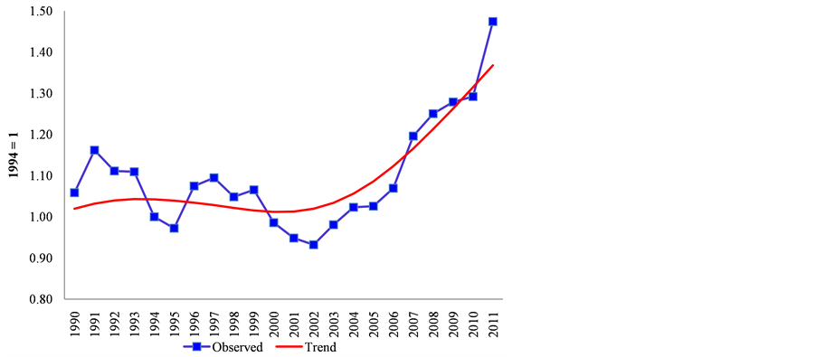
Figure 1. Average land productivity (1990-2011).
It is surprising to find out that a small share of total agricultural productivity gains are coming from “withinstate-within-crop” productivity changes (producing higher yields of a particular crop in one same state). Some have argued that this should be no surprise, since it is often the case that, in this sector, productivity increases of this sort tend to be slow, or at least slower than in other sectors of the economy, see Matusayama [19] . Others suggest that problems with land tenure, in particular “ejido” and its intrinsic weak property rights disables farmers to use the land lot as a collateral for accessing the credit market; at the same time, that these land lots are on average small enough to make capital investments not profitable, see Mackinlay and de la Fuente [20] , Dell [21] and Janvry, Emerick, González-Navarro & Sadoulet [22] . Others have blamed bad governmental policies, more focused on alleviating short term poverty issues than in solving the structural problems that the sector faces such as lack of infrastructure, sectoral organization, and so on, see Gómez-Oliver [11] , Yunez and Taylor [23] , Prina [24] and Aaragón & Campos [25] .
Recall that the “between-crop-effect” captures gains from the changes in shares of land used between existing crops. This term accounts for around 23 percent of the total changes in productivity, which means that-on average-land reallocation has favoured higher productive crops. In the same line, entrant crops are responsible of 4 percent of the national productivity increases and exiting crops were responsible of around 2 percent of total increases in productivity. This shows that in order to increase output value it is not only important to cultivate and harvest more but that selection of crops matter too (in fact land cultivated does not increase in the period where output value increases).
What Crop Groups Are Really Driving Productivity Growth?
NAFTA stipulated five year tariff elimination phases, and it is in the year 2003 when many agricultural tariffs were eliminated. In particular, The United States lifted tariff restrictions to several goods falling into the two digits Harmonization System “07” and “08”, that is “Vegetables” and “Fruits, nuts, citric and melons”, respectively. According to data reported by INEGI, these two groups—that account to nearly 80 percent of agricultural exports—exhibit an acceleration in export value growth from the year 2003 and continue growing throughout the rest of the period; something that could be explaining the better performance of the sector in this second half8. Figure 2 plots export values of the crop groups mentioned.
In addition, most of the crops that expanded their land shares or entered the production market are high productive crops and are likely to be linked to the export market. For example, data shows that 15 out of the top 20 fastest growing crops—in terms of land share—fall into the “Vegetables” and “Fruits, nuts, citric and melons” crop groups, while 4 or the remaining 5 fall into crops considered as “forage”. On the contrary, the biggest “losers” in terms of land share were mostly import competing crops (“Maize’’, “Barley” and “Wheat”). Notice, from Figure 3, that agricultural exports have grown at a faster rate than overall agricultural output, see Figure 3.

Figure 2. Exports of “vegetables” and “fruits, nuts, citric and melons”.
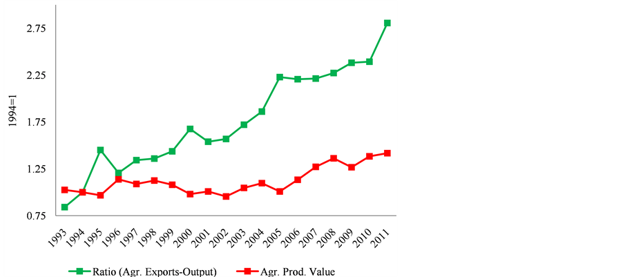
Figure 3. Agricultural exports as a share of output.
From Table 1, it can be seen that the largest share of productivity changes comes from the group “Cereals”; however, this is also the biggest agricultural group at the national level (both in terms of land cultivated and output value), so the result might not be surprising. However, observe that the group “Edible fruits and nuts, peel of citrus/melons” were responsible of over 24 percent of the changes in productivity; despite the fact that this group makes use of only 7 percent of the total agricultural land in the country (thus contributed the most per hectare harvested). Something similar occurs with the group “Edible vegetables” that account for less than 10 percent of land cultivated but over 27 percent of total productivity changes, as well as “Oil seeds, misc. grains, medicinal plants”. This is the result of the fact that these crop groups had higher initial productivity levels, have seen it grow and have also increased their share of land cultivated over the period. The rest of the groups have contributed negatively to national productivity, given their low initial productivity levels, accompanied in some cases to falling productivity. Importantly, we find that these last groups have shrunk in size in the period of study.
6. Discussion
We have studied the behaviour of diverse variables regarding the Mexican agricultural sector between the years of 1990 and 2011. This has been done with the idea of understanding the evolution of agricultural land productivity and the sources behind its growth. Results emphasize the importance of land reallocation dynamics.
During the first half of the period of study, agricultural land productivity shows no growth, but from the year 2003 it starts growing consistently and, as a result, production value grows too. The relationship between productivity and production value is evident given that total land harvested does not increase in the period where production value does. The rise in productivity growth in the latter half of the period is important. While national land productivity levels in the year 2002 were below those of 1990, after that year productivity rose at an average rate slightly above 5 percent annually. Results show that a large share of productivity changes were due to different kinds of land reallocation, in particular, reallocation “between-crops” and “across-states”.
Specifically, estimations show that nearly 80 percent of the land productivity changes over the period were due to “within-crop” productivity changes. That is, to the improvement in hectare-productivity value across crops. Additionally, we have found that nearly 70 percent of this term was due to crop-production shifts towards relative “crop-productive” states. Leaving the rest to “within-state-within-crop” productivity changes, which are improvements in crop productivity across states per-se.
On another count, measurements show that 23 percent of overall productivity changes are due to changes in land use in terms of crop selection. A process that favoured on one side productive export-oriented crops that fall in the “HS” classifications of “Fruits, & Nuts, peel of citrus and melons” and “Edible vegetables” and on the other side relative unproductive “Forage” crops. These findings are relevant both because they give information about what is driving agricultural land productivity changes in Mexico and is likely to be happening in its own terms to other developing countries in the face of free trade. They also suggest that trade liberalization has played a key role in shaping production patters in Mexico. Both “between-crop” reallocation and “betweenstate-crop” reallocation dynamics support the comparative advantage theory of trade. Given that the direction of changes in land use has favoured productive export oriented crops. These terms together account for more than three quarters of overall productivity growth during the period.
While it is true that the agricultural sector has shown signs of improvement over the last decade, the sector starts from a low base and it is still a vulnerable sector; in particular given the failure to transit to a more competitive level with a larger share of land devoted to export oriented crops instead of import competing crops where Mexico does not hold comparative advantages. This is a critical consideration given the enormous share of agricultural land that is devoted to relatively unproductive crops. There exists huge opportunities to exploit price differentials between countries, to do so the country must take advantage of resource endowed comparative advantages9.
Studies suggest that this sector has lagged for not being able to successfully adapt to changing circumstances (due to rural poverty, strong credit constraints, lack of market information, technical assistance and to bad organization between producers that together translate into important production and commercialization barriers). Strengthening the sectoral integration could result in the surge of commercialization and production networks, important for the incorporation of the sector to international markets10. Given the high levels of poverty, that in many cases impede farmers to overcome these obstacles; it seems necessary that governmental policy plays a better and stronger role in filling these holes if the country is to take advantage of the potential increases in trade flow that could exist11.
While it is true that under any trade liberalization there will be “winners” and “losers”. Mexico needs to adopt and grow its “winners” by transforming the production of non-competitive crops into self-sustainable crops in the international game. Without a true transformation of the sector towards the crops in which Mexico has comparative advantages, it seems hard to think the sector will survive in the “long-run” without fiscal support in form of non-productive subsidies.
References
- Tornell, A., Westermann, F. and Martinez, L. (2004) NAFTA and Mexico’s Less than Stellar Performance. NBER, Working Paper 10289.
- Gordon, H.H. (2010) Why Isn’t Mexico Rich? Journal of Economic Literature, 48, 987-1004
- Kehoe. T.J. and Ruhl, K.J. (2010) Why Have Economic Reforms in Mexico Not Generated Enough Growth. National Bureau of Economic Research (NBER). Working Paper 16580.
- Levy, S. and van Wijnbergen, S. (1995) Transition Problems in Economic Reform: Agriculture in the North American Free Trade Agreement. The American Economic Review, 85, 738-754.
- Lewis, W.A. (1954) Economic Development with Unlimited Supplies of Labour. The Manchester School of Economic Social Studies, 22, 139-191.
- Ray, D. (1998) Development Economics.1st Edition, Princeton University Press, New Jersey.
- Narro Robles, J., Navarro, D.M. and de la Fuente Stevens, D. (2013). Desafíos y descalabros de la política social en México. Problemas del Desarrollo, 174, 9-34.
- Verhoogen, E.A. (2008) Trade, Quality Upgrading and Wage Inequality in the Mexican Manufacturing Sector. Quarterly Journal of Economics, CXXIII.
- Marañón, B. and Fritscher, M. (2004) La agricultura mexicana y el TLC: El desencanto neoliberal. Debate Agrario, 183-210.
- Yunez, N. (2012) The Effects of Agricultural Domestic and Trade Liberalization on Food Security: Lessons from Mexico. Working Paper. Colegio de México, Colmex.
- Gómez-Oliver, L. (1996) El papel de la agricultura en el desarrollo México. Revista de estudios agrarios, No. 3, (abril-junio), Procuraduría Agraria, México.
- Foster, L., Haltiwanger, J.C. and Krizan, C.J. (2001) New Developments in Productivity Analysis, Chapter 8, 303-372. University of Chicago Press, Chicago, NBER.
- Bertelsman, E., Haltiwanger, J. and Scarpetta, S. (2004) Microeconomic Evidence of Creative Destruction in Industrial and Developing Countries. Discussion Paper Series IZA, No. 1374.
- Krugman, P. and Obstfeld, M. (2006) International Economics: Theory and Policy. 7th Edition, Pearson—Addison Wesley, Boston.
- Pavcnik, N. (2002) Trade Liberalization, Exit and Productivity Improvements: Evidence from Chilean Plants. NBER, Working Paper Series.
- Helpman, E. (2004) The Mystery of Economic Growth. Harvard University Press, Cambridge.
- Melitz, M. (2003) The Impact of Trade on Intra industry Reallocations and Aggregate Industry Productivity. Econometrica, 71, 1695-1725.
- Jones, C.I. (1998) Introduction to Economic Growth. 2nd Edition, W. W. Norton & Company, New York,
- Matusayama, K. (1992) Agricultural Productivity, Comparative Advantage, and Economic Growth. Journal of Economic Theory, 317-334.
- Mackinlay, H. and de la Fuente, J. (1996) La nueva legislación rural en México. Debate Agrario, 73-95.
- Dell, M. (2011) Insurgency and Long-Run Development: Lessons from the Mexican Revolution. Unpublished.
- de Janvry, A., Emerick, K., González-Navarro, M. and Sadoulet, E. (2012) Certified to Migrate: Property Rights and Migration in Rural Mexico. Unpublished.
- Yunez, N. and Taylor, E. (2006) The Effects of NAFTA and Domestic Reforms in the Agriculture of Mexico: Predictions and Facts. Région et Développment, 161-188.
- Prina, S. (2007) Agricultural Trade Liberalization in Mexico: Impact on Border Prices and Farmers’ Income. Boston University-Department of Economics.
- Aaragón, E., Fouquet, A. and Campos, M.. (2009) The Emergence of Successful Export Activities in Mexico: Three Case Study. Inter-American Development Bank, Research Network Working Paper No-R555.
- Rodrik, D. (2004) Industrial Policy for the Twenty-First Century. John F. Kennedy School of Government, Harvard University.
Appendix
In this section we will derive Equation 3.
Define “I” to all element 
Define “x” to all element 
Define “n” to all element 
where  and
and 
If we assume that  and that
 , then
 . Such that we can define sectoral productivity as a weighted average of crop productivity in the following way:

Then, if we leave aside the assumption and we take –as happens in the data that  and that
 ; we must add the last two terms of the next equation for the equality to hold.

NOTES

1While in the 1970s decade this sector represented around 20 percent of national GDP and over 60 percent of exports, in the year 2011 it contributed with little less than 4 percent of GDP and 2 percent of exports. Today, Mexico has a trade deficit in the agricultural products.
2INEGI is the Mexican, federally funded, institution of national statistics.
3CONEVAL is the Mexican governmental agency in charge of measuring poverty and evaluating social policy.
4This result is mainly driven by the fact that the crop “maize”, the largest agricultural product in Mexico falls into this group. Despite the fact that it has been shrinking in terms of the share of total land used over the last twenty years, it still uses little more than 35 percent of the total land harvested in Mexico. Nonetheless, in 2010 it only represented around 20 percent of the total output value.

5Gómez-Oliver estimates that the average import tariff fell from 27 to 10 percent and that the import permits were lowered from 92.2 percent in June of 1985 to less than 18 percent by the end of 1990.
6Own translation from the text.

7To see the derivation of Equation (3) see Appendix.

8Yunez-Naude estimated that after NAFTA Mexican Agricultural exports to its northern neighbour accounted for over 95 percent of its total agricultural exports.

9While the share of land devoted to “Cereals” excluding the ones of `forage’ use have fallen over the last decade they still constitute a dominant share of agricultural land. The most notorious case is the crop “maize” which represents around 35 percent of the total land harvested, but only 20 percent of the production value.
10Something that has happened already in isolated cases like the “avocado”, where Mexico rapidly became the largest producer and exporter of the fruit. See Aaragón, Fouquet & Campos .
11See Rodrik for examples where governmental support policies has led to the notable surge and expansion of industries around the globe.