Theoretical Economics Letters
Vol. 2 No. 2 (2012) , Article ID: 19286 , 5 pages DOI:10.4236/tel.2012.22027
Stationary Vector Autoregressive Representation of Error Correction Models
Department of International Trade, Dankook University, Yong-In, Korea
Email: yunyeongkim@dankook.ac.kr
Received December 16, 2011; revised January 20, 2012; accepted January 28, 2012
Keywords: VAR Model; Cointegration; Error Correction Model; Stationary VAR
ABSTRACT
The paper introduces a stationary vector autoregressive (VAR) representation of the error correction model (ECM). This representation explicitly regards the cointegration error a dependent variable, making the direct implementation of standard dynamic analyses using standard VAR models possible, particularly with respect to the cointegration error. Of course, an ECM does not have an explicit VAR form, and thus, it is not convenient for conducting such dynamic analyses. In this regard, we transform the original nonstationary VAR model into a VAR model with the cointegration error and stationary variables. Finally, we employ the model to dynamically analyze the real exchange rate between the US dollar and the Japanese yen.
1. Introduction
The dynamic analysis of the cointegration error and stationary variables in the short run is important as the longrun equilibrium for practitioners and policy makers. Of course, such work is possible through the classical error correction model (ECM), which was popularized by Engle and Granger (1987). Furthermore, the persistence profiles of Pesaran and Shin (1996) and Hansen (2005) are also useful alternatives for this purpose.
Another possible option is to follow the vector autoregressive (VAR) approach of Sims (1980), which is now a standard method. In particular, such work may be possible if we transform the ECM into a VAR form of the cointegration error and stationary variables, which would allow the more direct exploitation of the rich tools of VAR analyses (i.e., the Granger causality test, impulse response analysis, variance decomposition, and optimal forecasting). Obviously, an ECM does not have an explicit VAR form, and thus, it is not convenient for conducting such dynamic analyses.
Then the question is whether we can transform the ECM into a finite-order VAR model of the cointegration error and stationary variables. In this regard, this paper derives a finite-order VAR model with the cointegration error that is conformable to the ECM for the short-run adjustment. In the VAR model, the cointegration error is regarded as a dependent variable, and VAR-type dynamic analyses may be conducted directly.
Finally, we employ the model to dynamically analyze the real exchange rate between the US dollar and the Japanese yen.
The rest of this paper is organized as follows. Section 2 introduces the model and assumptions. Section 3 discusses on the stationary VAR model representation of ECMs. Section 4 presents the empirical results, and Section 5 concludes.
2. Model and Assumptions
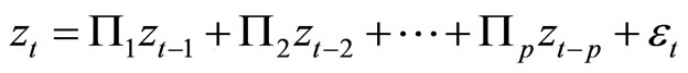
We consider the  -dimensionaland integrated of one VAR(p) process of
 ![]() given by
given by
 (1)
(1)
or
 (2)
(2)
where
 ,
,
and  is an
is an  vector of an independently and identically distributed disturbance term with a finite variance
 , where
  denotes an
  -dimensional identity matrix and
 .
.
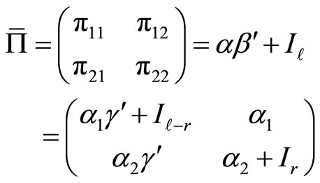
Further we assume the cointegration of Model (1) (e.g., Johansen, 1995) as:
Assumption
We suppose , where
 ![]() and
and  are
are  matrices of the full-column rank
 .
.
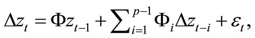
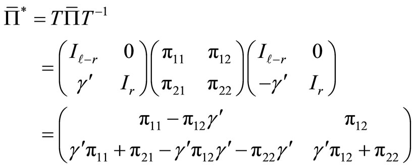
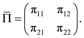
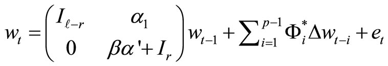
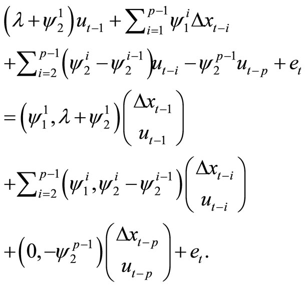
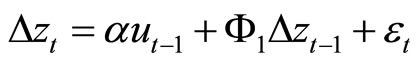
Note that Model (2) may be written in an ECM as
 (3)
(3)
under Assumption 2.1, where .
.
Model (3) obviously consists of all stationary variables of  and
and  under Assumption 2.1. We are now interested in the dynamic interaction between these variables
  and
and . In this regard, we may apply the results of Pesaran and Shin (1996) and Hansen (2005). However Sims’ (1980) VAR approach is sometimes convenient for practical reasons. For instance, the optimal forecasting of the k-th-period-ahead cointegration error
  is executed mechanically in a VAR system.
Thus, we now show that Model (3) may be represented as a stationary VAR model of a part of variables  and
and  when there is an ECM.
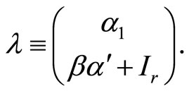
3. Stationary VAR Representation of ECM
To obtain a stationary VAR representation, assume that a given cointegration vector is normalized as 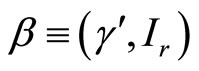 of the rank
 , where
  is
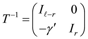
is . Then a confirmable non-singular square matrix can be defined as
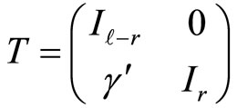
![]() .
.
Noteworthy is that the above lower triangular matrix  transforms the VAR variable
  into a variable
  of
of  and cointegration error
 .
.
 .
.
Note that  is the explanatory variable of
  in a cointegration relation as
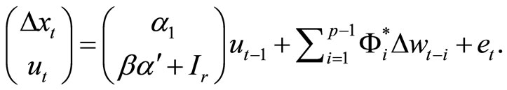
 .We then transform the above VAR model (1) of
 ![]() into a VAR model of the variable
into a VAR model of the variable . In particular, we multiply the
 ![]() on the left of Model (1) and modify the VAR coefficients to get the following VAR model:
on the left of Model (1) and modify the VAR coefficients to get the following VAR model:
 (4)
(4)
where  for
for  and
and .
.
Note that Model (4) is an observationally equivalent form of Model (1) or (3) if  has a Gaussian distribution. However, we cannot determine the correct model by simply analyzing observed data.
Then it is helpful to write Model (4) as
 (5)
(5)
where  and
and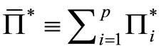 .
.
Then we may simply arrange  in Equation (5) as follows:
3.1. Proposition
Suppose that Assumption 2.1 holds. Then
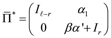
where  is
is ,
,  is
is  and
and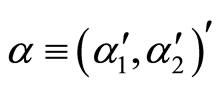 .
.
Proof of Proposition 3.1. We first write from the definition
 (6)
(6)
by using
for the first equality, where
We now represent the submatrices of  in the third equality of (6) by using
 ![]() and
and , where
  under Assumption 2.1. For this, note that
 (7)
(7)
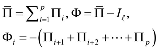
because the matrix Φ can be written as
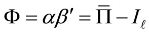 (8)
(8)
from the coefficient definition of (2) for the second equality.
Then the third equality in Equation (7) directly implies that
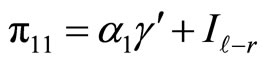 (9)
(9)
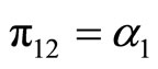 (10)
(10)
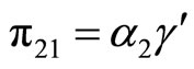 (11)
(11)
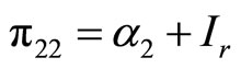 . (12)
Consequently, if we plug the submatrices (9)-(12) into the last term in Equation (6), then we get following:
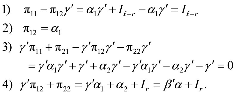
The above results 1)-4), together with the equality in (6), proves the claimed result as
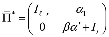
from (6). ■
Note that both the dependent and explanatory variables in (5), have the nonstationary variables  and
and  in
in  and
and . Thus, we show how we may transform Model (5) of
  into a VAR model of a purely stationary variable
 .
.
3.2. Theorem
Suppose that Assumption 2.1 holds. Then
 (13)
(13)
where 
for i = 2, 3,···, p − 1 and  and
and  .
.
Proof of Theorem 3.2. Using Proposition 3.1, we first rewrite Model (5) as
or
 (14)
(14)
The right hand side of (14) may be written as
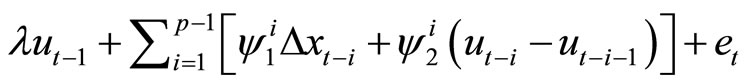 (15)
(15)
defining
Finally, the term in (15) may be written as
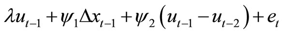
Thus, Model (14) may be rewritten as a p-th order VAR model of :
:
 (16)
(16)
Note the restrictions

 (17)
(17)
are imposed on  from Theorem 3.2, and
  does not appear in Equation (13). If these restrictions (17) are not exploited and the coefficients
  is estimated with errors, then the efficiency of dynamic analyses by using these estimated coefficients may be reduced. For instance, if we provide forecasts using a VAR model, then forecasting mean squared error may be increased not by using restrictions (17). Campbell and Shiller (1987, Equation (5)) used the system (13) without referring to the VAR model (1) of level variable
![]() , the rank deficiency of matrix
, the rank deficiency of matrix  in Assumption 2.1, and the restriction of Theorem 3.2 as
  of the coefficient
 .
.
Further, note that the vector moving average model of  is defined as
 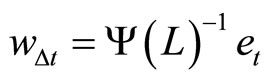 from (13) if
  is invertible, where L denotes a time-lag operator and
  This is conformable to the result in Hansen (2005, Corollary1).
In the following example, we transform an ECM into a VAR model of stationary variables.
3.3. Example
For a VAR (2), an ECM representation can be given as
 (18)
(18)
under Assumption 2.1. The second-order VAR representation of  is also possible as
 (19)
(19)
from Model (14) by using Proposition 3.1. The righthand side of (19) may be written as
 (20)
(20)
defining  conformably and
Finally, the term in (20) may be written as
Thus, Model (19) may be rewritten as a second order VAR model of :
:
 (21)
(21)
where and
and  conformably, where
 . Thus
  does not appear in Equation (21). Thus, the ECM (18) is written as a stationary VAR (2) model, as in (21). ■
Now any standard dynamic analysis is possible by using Model (13). Note that avariable  for
for  is known as long as the cointegration vector
  (and thus
 ) is known. Thus we may consistently estimate coefficients
  in Model (13) as
  with variables
 , using ordinary least square (OLS) method. However remind that the variable
  should be excluded from this regression.
Then we may conduct standard dynamic analyses by using the VAR model
where
 .
.
Suppose cointegration vector  is not known and estimated as
  with super-consistency as
  [c.f., Johansen (1995)] where n is a sample number. Then
  should be replaced by
 where
where . Thus we may consistently estimate coefficients
  in Model (13) as
  with variables
  by using the OLS, where the variable
  should be excluded from the regression. Finally, we may conduct standard dynamic analyses by using the VAR model
where
In this case, we may still conduct standard dynamic analyses and draw inferences from stationary VAR analyses because  may be considered as known
  because of its rapid convergence. See Hamilton (1994) for a nice review on this issue.
4. Application: An Impulse Response Analysis of the Real Exchange Rate
The US is highly concerned about the potential exchange rate manipulation by East Asian countries for their trade
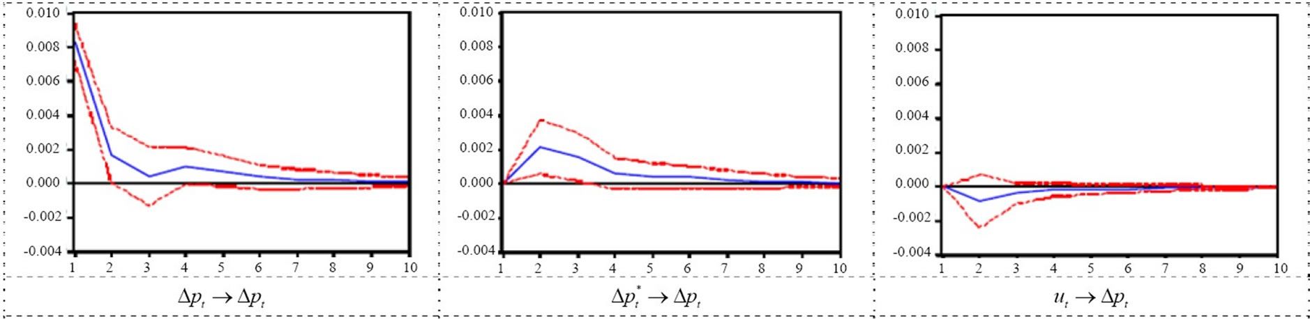
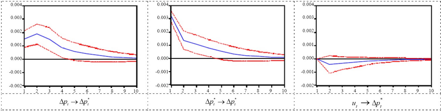
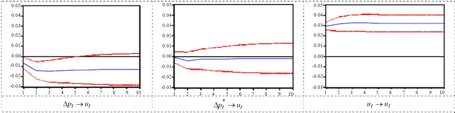
Figure 1. Impulse response analysis for USA-JAPAN PPP (response to cholesky one S.D. innovations ± 2 S.E.).
surplus. Krugman and Baldwin (1987) provide a classic study of this issue. See also Clarida and J. Gali (1994). The logic behind this manipulation can be explained by the law of one price (LOOP). Let ,
,  and
and  denote the log of the price level in the US (
 ), the log of the Japanese price level (
 ), and the nominal yen/dollar exchange rate (
 ), respectively. The LOOP states that
  and that the same goods should be sold at the same prices both at home and in foreign countries, where prices are converted into local prices at prevailing exchange rates. Here if the exchange rate
  is manipu lated as
  through state intervention, then it is possible that
  in the short run, where
  is the relative price of the foreign good. Then the cheaper price of the home country good may induce a trade surplus.
Then the question is whether any exchange rate or price shock would have a statistically meaningful effect on the real exchange rate (a cointegration error if the real exchange rate is I(0)). To address this question, we construct a VAR model of 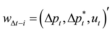 in (13), where
 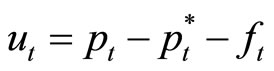 and
and .
.
Finally, we conduct an impulse response analysis on  by using the Model (13). An ECM (3) does not have an explicit VAR form, and thus, it is not convenient for conducting such impulse response analysis. For this, we employ monthly data for the period from January 1998 to December 2008. We excluded the recent global financial crisis because of a possible structural break.
We conduct unit root tests for the variables ,
, 
 and
and . The results of the KPSS test do not reject the null hypothesis of stationarity at the 1% level for the cointegration error
  in the yen/dollar exchange rate. However, the null hypothesis of a unit root cannot not be rejected for the other variables. In a VAR model of
 , we obtained order 2 by using the Akaike information criterion, and the results of the Johansen test reject the null hypothesis of no cointegration at the 1% level. The possible number of ordering for the identification of structural shocks is 6 for the trivariate model, and we investigate all these cases. However, changing the order has no influence on the results. Thus, we report only the result for the identification order
  . The impulses from the US price and the yen/dollar exchange rate have significant effects on the Yen/Dollar real exchange rate. See Figure 1 for the results of the impulse response analysis.
5. Conclusion
The ECM is clearly one of the most powerful methods in econometrics. However, it does not have an explicit VAR form with the cointegration error as a dependent variable. This paper introduces a stationary VAR representation of the ECM that explicitly regards the cointeration error as a dependent variable, making the direct implementation of standard dynamic analyses using stationary VAR models possible, particularly with respect to the cointegration error.
6. Acknowledgements
I am grateful to Joon Y. Park, Byeongseon Seo and the anonymous referee for their invaluable comments. All remaining errors are the author’s own.
REFERENCES
- J. Y. Campbell and R. J. Shiller, “Cointegration and Tests of Present Value Models,” Journal of Political Economy, Vol. 95, No. 5, 1987, pp. 1062-1088. doi:10.1086/261502
- R. Clarida and J. Gali, “Sources of Real Exchange Rate Fluctuations: How Important Are Nominal Shocks?” NBER Working Papers No. 4658, 1994.
- R. F. Engle and C. W. J. Granger, “Co-Integration and Error Correction: Representation, Estimation, and Testing,” Econometrica, Vol. 55, No. 2, 1987, pp. 251-276. doi:10.2307/1913236
- J. D. Hamilton, “Time Series Analysis,” Princeton University Press, Princeton, 1994.
- P. R. Hansen, “Granger’s Representation Theorem: A Closed-Form Expression for I(1) Processes,” Econometrics Journal, Vol. 8, No. 1, 2005, pp. 23-38. doi:10.1111/j.1368-423X.2005.00149.x
- S. Johansen, “Likelihood-Based Inference in Cointegrated Vector Autoregressive Models,” Oxford University Press, New York, 1995. doi:10.1093/0198774508.001.0001
- P. R. Krugman and R. E. Baldwin, “The Persistence of the US Trade Deficit,” Brookings Papers on Economic Activity, Economic Studies Program, The Brookings Institution, Washington, 1987, pp. 1-56.
- M. H. Pesaran and Y. Shin, “Cointegration and Speed of Convergence to Equilibrium,” Journal of Econometrics, Vol. 71, No. 1-2, 1996, pp. 117-143. http://dx.doi.org/10.1016/0304-4076(94)01697-6.
- C. A. Sims, “Macroeconomics and Reality,” Econometrica, Vol. 48, No. 1, 1980, pp. 1-48. doi:10.2307/1912017