ABSTRACT

We applied two daily average temperature models to Canadian cities data and derived their derivative pricing applications. The first model is characterized by mean-reverting Ornstein-Uhlenbeck process driven by general Lévy process with seasonal mean and volatility. As an extension to the first model, Continuous Autoregressive (CAR) model driven by Lévy process is also considered and calibrated to Canadian data. It is empirically proved that the proposed dynamics fitted Calgary and Toronto temperature data successfully. These models are also applied to derivation of an explicit price of CAT futures, and numerical prices of CDD and HDD futures using fast Fourier transform. The novelty of this paper lies in the applications of daily average temperature models to Canadian cities data and CAR model driven by Lévy process, futures pricing of CDD and HDD indices.

1. Introduction

Over the last decade, weather derivatives have emerged as an attractive and interesting new derivative class for risk management and other related fields. Since the purpose of weather derivatives is to allow businesses and other organizations to insure themselves against fluctuations in the weather, a number of insurance, reinsurance companies, banks, hedge funds and energy companies have set up weather trading desks. It is obvious that there are close connections between energy and weather, for example, a natural gas distributor may want to buy weather derivatives to ensure profits in case of a warm winter in which consumers will buy less gas for heating purpose. Hence, weather derivatives will provide a financial instrument for companies or organizations to avoid some unzealous impact of the “bad” weather effects and control the weather risks. Also, additional instruments for hedging in the energy markets require quantitative models of both energy and weather derivatives included.

The weather derivatives market, in which contracts written on weather indices was firstly appeared Over-thecounter (OTC) in July 1996 between Aquila Energy and Consolidated Edison Co. from United States. After that, companies accustomed to trading weather contracts based on electricity and gas prices in order to hedge their price risks realized by weather during the end of 1990s and the beginning of 2000s. Consequently, the market grew rapidly and expanded to other industries and to Europe and Japan. Reported from Weather Risk Management Association (WRMA), an industry body that represents the weather market, recently, the total notional value of the global weather risk market has reached $11.8 billion in last year. With geographic expansion, the OTC market boosted nearly 30% in last year. In this article, we will concentrate on the futures market of temperature derivatives found at the Chicago Mercantile Exchange (CME), which is one of the largest weather derivatives trading platforms. Up to now, the CME has weather futures and options traded based on a range of weather indices for 47 cities from United States, Canada, Europe, Australia and Asia.

As a common sense, weather affects different entities in different ways. In order to hedge these different types of risks, weather derivatives are written on different types of weather variables or weather indices. The most commonly used weather variable is the temperature. Widely used temperature indices include cumulative average temperature (CAT), heating degree days (HDD) and cooling degree days (CDD). They are originated from the energy industry, and designed to correlate well with the local demands for heating or cooling. CAT are defined as the sum of the daily average temperature over the period of the contract, the index

where is the daily average temperature. It is mainly used in Europe and Canada. In winter, HDD are used to measure the demand for heating, i.e. they are a measure of how cold the weather is and usually used in United States, Europe, Canada and Australia. In contrast, CDD are used in summer to measure the demand of energy used for cooling and a measure of how hot the weather is. They are usually used in United States, Canada and Australia. The definitions for HDD and CDD are given by

andwhere the threshold takes value of.

The pricing of a given weather derivative by calculating the expected value of its appropriately discounted payoff is inherently related to weather forecasting and simulation (see Zeng [1] and Cao and Wei [2]). The conventional approach is to identify the probability distribution of the associated index at maturity, and then integrate the payoff of the derivative with respect to it. Dornier and Queruel [3] characterized weather dynamics by mean-reverting Itô diffusions, driven by a standard Brownian motion, and then resorted to Monte Carlo simulation. Davis [4] used the geometric Brownian motion to model the accumulated HDDs (or CDDs). Brody et al. [5] proposed to replace the traditional Brownian motion by a fractional Brownian motion, leading to a fractional Ornstein-Uhlenbeck, allowing incorporate a long memory effect. Benth [6] used the Fourier transformation technique to get the explicit expressions of European and average type of weather contracts, and also showed the pricing formulas satisfy certain Black-Scholes PDE. Benth and Šaltytė-Benth [7] proposed an Ornstein-Uhlenbeck model with seasonal mean and volatility, where the residuals are generated by the class of generalized hyperbolic Lévy process rather than Brownian motion family. The process they used is a flexible class of Lévy process capturing the semi-heavy tails and skewness properties of residuals. A similar model driven by Brownian motion was applied for pricing CAT, HDD and CDD futures in Benth and Šaltytė-Benth [8], they also gave discussions about options written upon these futures. Benth et al. [9] generalized the analysis in the above OU model to higher-order (with lag p) Continuous-time Autoregressive models with seasonal variance for the temperature, and they found the choice of p = 3 turns out to be sufficient to explain the temperature dynamics in Stockholm, Sweden by calibrating the model to more than 40 years of daily observations. More recently, Zapranis and Alexandridis [10] began proposing using a time dependent speed of mean reversion parameter in the Ornstein-Uhlenbeck model and use neural networks to estimate the parameters.

The remaining of this article is organized as follows: In Section 2, we firstly apply existed Lévy driven meanreverting model to the modeling of temperature index of Canadian temperature data, and then present Lévy driven CAR model and its application to Canadian data. In Section 3, we develop the futures pricing techniques with respect to weather futures of CAT, CDD and HDD based on the established two models. Finally, in Section 4, we illustrate the concluding remarks and some possible future research in this direction.

2. Modeling of Weather Index

2.1. Lévy Driven Ornstein-Uhlenbeck Model

As our first proposed model, consider the weather index, which is the daily average temperature (DAT). We suppose the DAT has a generalization of the dynamics:

(1)

where is the seasonal mean level across years given days and is the speed in which revert to. is assumed to be a measurable and bounded function represents the seasonal volatility of temperature. is cádlág, adapted, real valued Lévy process with independent, stationary increments and stochastically continuous. For formal definition of Lévy process, we refer the reader to the introduction paper by Papapantoleon [11]. This model was firstly introduced by Dornier and Queruel [3] with Brownian motion. We will firstly apply this model with Lévy process to Canadian temperature data.

From Equation (1), we can directly use Itô formula for semimartingales to get the explicit solution

(2)

For the purpose of fitting this model to our daily average temperatures, we reformulate Equation (2) by subtracting from,

(3)

with the notation. The stochastic integral could be approximated by

(4)

Adding to both sides

(5)

If we define, we will have the following three parts for modeling step by step:

(6)

where is the seasonal component, is the cyclical component derived from Equation (5), and is the stochastic part.

The data sets we are going to analyse include daily average temperatures (measured in centigrade) from Calgary, AB and Toronto, ON in Canada. The choice of these two cities is intuitively based on the location and importance of these cities. These data are provided by the Canadian National Climate Data and Information Archive (NCDIA) over a period ranging from January 1^st 2001 to January 1^st 2011, resulting in 3652 records for each city. For simplicity, the measurement on each February 29^th was removed from the sample in each leap year to equalize the length of each year.

2.1.1. Linear Trend

Empirically, the daily average temperature should have an increasing trend due to some reasons such as global warming, green-house effect and so on. However, from Figure 1, we cannot verify significant linear trends for both data sets. The slopes for linear fitting of Calgary and Toronto are and respectively. A potential explanation to this is that our sample size is reasonably small with a period of 10 years data. Larger sample size will show us relatively more significant increasing trend using least square fit. Hence, at this stage we will ignore the linear trend, and keep a constant mean level in the seasonal trend.

2.1.2. Seasonal Trend

In order to model the seasonality pattern, we use the trigonometric function with the form

(7)

where is the mean level, is amplitude of the mean. The period of the oscillations is one year (365 days neglecting leap year), so the weight.

represents the phase angle. The results of parameters estimation using least square method are reported in Table 1.

2.1.3. Cyclical Component

To remove the adjacent correlation in the time series, make the time series stationary, we model the cyclical component by recursive regression based on Equation (5). The cyclical componentcan be modeled by:

(8)

The results ofestimated implicitly by an autoregressive model and correspondingare given in Table 2.

The autocorrelation function (ACF) plots for the squared residuals in Figure 2 clearly reveal seasonality of correlation for both cities. In the squared residuals ACF plots, the autocorrelation violated interval for lots of lags, and the wave for the ACF is a sign of

Table 1. Estimated parameters for seasonal function.

Table 2. Estimated parameters in regression.

seasonal pattern.

2.1.4. Seasonal Volatility

We consider the seasonal pattern in the residual after removing the cyclical component as the seasonal volatility. The motivation behind seasonal volatility is straight forward. The temperature appears bigger variation in the winter and smaller variation in the summer. By Equation (5), the random term has the form. To get the seasonal volatility, we have the following methods:

• Organize the data into 365 groups, one for each day of the year;

• Find the means of the squared data in each group. These means are crude estimation for the expected squared data.;

• To smooth the estimation, first way is trying the smoothing technique. In details, we could take logarithm of the estimation and use moving average method to smooth the crude estimation. Then the smoothed estimation of could be get by ex-

ponentiation of the result. Alternatively, use the truncated Fourier series (9) to fit the estimation from previous two steps. The Fourier series will indicate the presence of different cycles in as a deterministic function.

(9)

Figure 3 shows the fitted and smoothed by three days moving average technique. More average smoothing range will make the estimation smoother, but for our Canadian temperature study, the variation of the temperature in more days would be relatively larger than that of three days. Hence, the choice of three days moving average makes sense for both the smoothing and accuracy purpose.

After removing the estimated seasonal volatility, the ACF for the data and squared data are plotted in Figure 4. It shows that the seasonality pattern is completely removed from the squared data.

On the other hand, we also tried the way of fitting the crude seasonal volatility by truncated Fourier series with other three. The values of the estimated parameters are given in Table 3.

Corresponding fitted results are shown in Figure 5.

Again, the seasonal pattern in the ACF plot was removed from Figure 6. So, we could find that both methods can model the seasonal volatility appropriately.

2.1.5. Random Noise

Then we head to fit the random part remained from

Table 3. Truncated fourier series parameters.

above. The classical literatures of temperature modeling suggest the random noise are independent and identically normal distributed, (see Dornier and Queruel [3], Alaton et al. [12]). However, we could see from the QQ-plot and normal fit of the random noise for our data, the normal distributed random noise may lead misdescription to the data. Moreover, modeling of random noise using Gaussian process is not always the case.

Instead, we try to apply the generalized hyperbolic family process to model the random part for our data, based on Benth and Šaltytė-Benth [7]. As the name suggests, it is super-class of processes such as normal-inverse Gaussian, variance-gamma, hyperbolic and so on. This will allow the family better capture the features of the data set and relatively easy to analyze from the Lévy properties it holds.

The generalized hyperbolic distribution is an infinitely divisible distribution which can be defined with the density function

where is modified Bessel function of the third kind with index. Parameters of the generalized hyperbolic distribution can be estimated by maximum likelihood method. In detail, for a vector of observations

, the maximum likelihood estimate of the parameters can be obtained by maxi-

mizing the log-likelihood function for generalized hyperbolic distribution:

McNeil et al. [13] described a modified EM method, which is called multi-cycle, expectation, conditional estimation (MCECM) algorithm to optimize the log-likelihood function. We use this algorithm written as “ghyp” package in “R” to estimate parameters. Estimated parameters are presented in Table 4.

In order to check the goodness of fitting, we simulated a series of generalized hyperbolic distributed random

Table 4. Estimations of generalized hyperbolic parameters.

variables using estimated parameters, and plotted the empirical cumulative distribution function, then compared with our residual observations’ empirical cumulative distribution function plot. The results are shown in Figure 7. The result implies our calibration to the model is reasonably fair for Canadian data.

2.2. Lévy Driven Continuous-Time AR Model

Another suitable class of stochastic process we could use to analyze the evolution of temperature is an extension of the previous OU process to the multi-factor OU process. The model is called Continuous-time Autoregressive (CAR) model, which is also a subclass of the general Continuous-time Autoregressive Moving-average (CAR-MA) model introduced by Brockwell and Marquardt [14]. The intuition behind using this model is the temperature memory is consistent with high-order AR model, and the seasonality of mean and volatility is also involved in the model. In other words, the CAR model combine the mean-reverting property of OU process and the memory of AR model together to better capture the features of temperature.

Followed by the classical stochastic assumption, suppose given a probability space. Let be a stationary solution to the stochastic differential equation in for

(10)

where the operatordenotes the differential operator with respect to, is the p-order differential operator and is 1-dim Lévy process. Let be a column vector defined as

We could also rewrite the Equation (10) in the statespace form.

(11)

(12)

The vector is usually recognized as state vector. The standard deviation of the noise is described by a continuous function, we usually refer the

function as the volatility of the process. The constant denotes the order of the CAR model.

Assume additionally the seasonal function is bounded and continuously differentiable on. The temperature dynamics is formulated by:

(13)

where is the first entry of the state vector in Equation (11). Note that for Equation (12), since we have the function to capture the deterministic temperature level, the OU process should ideally revert to zero. This is the main reason we have only the meanreverting rate but without level in dynamic of

Again, by using the Itô lemma for semimartingale, the explicit solution for the stochastic differential Equation (12) has the form

(14)

If we construct the expectation of the Wiener-Lévy integral in Equation (14) equals to zero (it is obviously true for the Itô integral in the special case), once all eigenvalues of the matrix have negative real parts, the process then have a mean equal to zero. We could still use simple intuition to have the idea, when eigenvalues of the matrix have negative real parts and take then the expectation goes to zero. This result implies the temperature dynamic on average will mainly depend on the seasonal function by Equation (13).

Notice that we could have a link point of view to this CAR model from the previous OU model. Consider CAR(1) model as an example. In this case, in Equation (12), the matrix will simply becomes a constant. The process and by Equation (14), the temperature dynamics

Our proposed CAR model is therefore consistent with the single-factor OU model and also satisfies the requirements of regression and mean-reverting properties. For simplicity of estimation, we connect our CAR model to the classical AR model. Benth et al. [15] (Lemma 10.2) provided an explicit way to find the relation between the coefficients in CAR model and in AR model by induction as

(15)

with coefficients and initially

Next, we will recap the calibration procedure to the same empirical Canadian daily average temperature data based on the CAR model.

2.2.1. Linear and Seasonal Trend

As we did for OU model in Section 2.1.2., we could combine the linear and seasonal trend in the OU model to construct the seasonal functionin CAR model as

(16)

The coefficients for trigonometric function in Equation (16) play the same role in Equation (7). Followed by the description of linear trend in Section 2.1.2., we eliminated the linear part in again for CAR model, and the fitted results for seasonal part are the same to that in Table 1.

2.2.2. Cyclical Component

The PACF plots in Figure 8 clearly show that the evolution of detrended temperature could be modeled by the classical AR(3) model. Motivated by the PACF plots, by Equation (15), we have

The estimated parameters are outlined in Table 5.

PACF plots in Figure 9 show the significant correlation in the first three lags is removed by regression, but still a distinct seasonality in the ACF plots of squared residuals.

2.2.3. Seasonal Volatility

For the CAR model, we will apply the truncated Fourier series in Equation (9) to model the seasonal volatility. We choose the degree N = 1 in Equation (9), since there is no significant improvement for the result by adding degree. The fitted parameters are shown in Table 6.

In Figure 10 we present the empirical and fitted, both of them show that the fluctuation in the cold season are considerably larger than that of the mild season.

Figure 11 tells us that seasonal pattern in the squared residual is removed successfully.

Table 5. Estimations of cyclical component.

Table 6. Truncated Fourier series parameters.

2.2.4. Random Noise

We try again apply the generalized hyperbolic process to model our random noise part. The method is the same to that for OU model. Table 7 shows the fitted parameters for our Canadian cities data.

Also as we did for OU model, we simulated a series of generalized hyperbolic random variables with estimated parameters, then compare the empirical CDF with that of historical data in Figure 12. The empirical CDF coincides with simulated CDF almost perfectly, so we may expect this model fairly well describe our Canadian temperature data.

3. Pricing of Weather Derivatives

In this section, we will derive the temperature futures prices written on CAT, CDD and HDD, which constitute the three main classes of future products at CME market.

3.1. Future Pricing of Lévy Driven OU Model

Consider the price dynamic of future written on CAT over specific time period with Firstlyassume the daily average temperature follows stochastic differential Equation (1) with being Lévy process and constant continuously compounding interest rate The future price at time based on CAT under risk-neutral probability measure will be adapted stochastic process satisfying

(17)

Table 7. Estimations of generalized hyperbolic parameters.

By adaption of the stochastic process with respect to measure the future price

(18)

To derive the explicit future price in Equation (18), we need to specify a risk-neutral probability measure However, the commodity market is typical incomplete market, since most of commodity trades impose big transaction and storage cost. For our case, the underlying temperature is even not possible to be stored and traded. These features break down the classical hedging approach used to derive the unique fair price of derivatives. Because of the incompleteness of the temperature market, any probability measure Q being equivalent to the real measure P is a risk-neutral measure. Next, following the analysis in Benth and Šaltytė-Benth [16], we will specify a class of risk-neutral measure via Esscher transform. Before using the Esscher transform, we need an integrable condition for the Lévy measure to ensure the existence of moments of underlying asset process.

Condition 1. [Benth et al. ([15], p. 74)] such that the Lévy measuresatisfies the integrable condition

(19)

almost surely.

The constant determines the order of the moment that is finite for the underlying process. With this condition, we recap the following results from several sources that we will use in our further analysis (see Section 3.2).

Lemma 1. [Benth and Šaltytė-Benth [16]] Let function be a bounded and measurable function and Condition 1 holds for then

(20)

where is the cumulant function of the Lévy process is the Lévy symbol defined by map such that the characteristic function of the Lévy process

Now assume is a measurable and bounded function. Let us consider the stochastic process

(21)

The probability measure can be defined by the Esscher transform

(22)

where is the indicator function over a probability space. Obviously this measure is equivalent to the real measure and transformed from the probability measure so an equivalent risk-neutral measure. A way to get a more flexible class of equivalent martingale measure is to use time varying when fitting the observed forward curve. Note that the market price of risk is represented by in this case.

Then, consider the existence of the fair forward price dynamics given by Equation (18). We need to have another condition such that

is finite almost surely.

Condition 2. [Benth and Šaltytė-Benth [16]] Assume a constant satisfies such that Condition 1 holds, then the price dynamics

almost surely.

With the existence of explicit risk-neutral probability measure and fair pricing technique, we could derive the following results for the future price written on CAT.

Lemma 2. [Benth and Šaltytė-Benth [7]] Given a measurable and bounded function the expectation of Lévy integral under risk-neutral measure over is

With these lemmas, we could get the explicit formula for the future price written on CAT.

Theorem 1. [Benth and Šaltytė-Benth [7]] The future price at time written on CAT index is given by

Next, for pricing of CDD and HDD futures, recall that the CDD and HDD over a measurable time is

Before introduce the pricing technique for the CDD and HDD future, we should notice that there is a parity relation between futures prices of CAT, CDD and HDD. This relation will help us to get one of future price of CDD or HDD, once we have the CAT future price and the other one of them.

Theorem 2. [Benth et al. ([15], p. 279)] The relation between futures prices of CAT, CDD and HDD is

(23)

With this theorem, we will focus on the pricing of CDD future, but the pricing technique for CDD future is also analogously applicable to HDD future.

Based on risk-neutral pricing theory, the CDD future price satisfies

with risk-free interest rate and risk-neutral measure Given the risk-neutral measure derived from Esscher transform, since the CDD future under the measure is adapted, the risk-neutral CDD future price is derived as

(24)

Theorem 3. [Benth and Šaltytė-Benth [7]] For

the logarithm of characteristic function of under measure is given by

(25)

where is the cumulant generating function of

This theorem provides us a way to get the characteristic function of Lévy integral of the type under the risk-neutral measure With the characteristic function, the pricing approach we could try is using the celebrated Fourier inversion theorem to get the numerical probability density function of under measure, and then using the density function to price CDD future.

Theorem 4. (Fourier Inversion Theorem) [Hewitt and Stromberg ([17], p. 409)] Let denote the cumulative density function of random variable the corresponding probability density function is integrable in Lebesgue sense, i.e. The characteristic function of is defined as

Then,

(26)

To calculate the probability density function from characteristic function, consider the density and the discrete Fourier transform (DFT)

We could use the trapezoid rule to approximate the integral in Equation (26).

(27)

where The last step of approximation is because when we take to be large enough, The purpose to have the upper bound of summation as is to match with the form of DFT.

Now we propose an approach to calculate the probability density function analytically based on the construction of Chourdakis [18]. Note that the application of DFT will result in a set of integral approximation which have the form of Equation (27) based on

Let then For the return values these values are setting to be also equidistant with the grid spacing By contrasting Equation (27) and DFT, we have

Then set the return grids

(28)

where is a parameter to control the return range. For the center returns around zero, we could set

With these settlements, from Equation (27), the probability density function has the form

(29)

where This summation has the form of DFT, could be computed efficiently.

Theorem 5. Numerically, the CDD future

where is given by Equation (29) and are constructed by Equation (28) in the approach of fast Fourier transform.

Proof. Recall the CDD future is priced by Equation (24). By Fubini theorem, the definition of expectation and property of Riemann integral,

3.2. Future Pricing of Lévy Driven CAR Model

Now we assume the temperature dynamic follows Lévy driven CAR model, introduced by Equations (11) and (12). The risk-neutral measure is given by Equation (22), and the Existences of futures prices for CAT, CDD and HDD are preserved under Condition 2.

Based on the derivation of futures prices of CAT, CDD and HDD indices under Lévy driven OU model, we have the following results for the futures prices of these indices under the Lévy driven CAR model.

Lemma 3. The cumulated temperature on the time interval under Lévy driven CAR model is

Proof. Integrating the original Equation (12) over the time interval we have

Then, by using the solution of Lévy stochastic model, Equation (14), Equations (11) and (13),

So, the result is proved.                       

Theorem 6. The future price of CAT

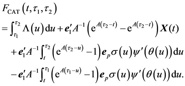
Proof. By Equation (18), we could use Lemma 3 to expand each term separately, and then use Lemma 2 to get the final explicit formula.                      

For CDD or HDD futures pricing, by using Theorem 3the characteristic function of could be found as where

Then, followed by the approach in the OU model, we have Theorem 7. Numerically, the CDD future price

where is given by Equation (29) and are constructed by Equation (28) in the approach of fast Fourier transform to compute

The proof of this theorem is similar to that of Theorem 5.

4. Summary, Conclusion and Future Work

This paper investigates the problem of modeling and pricing weather derivatives and their application to Canadian data. We have shown that two models, including Ornstein-Uhlenbeck model and Continuous-time Autoregressive model, both driven by Lévy process are fairly suitable to capture the evolution of Canadian cities temperature. Also, based on these two models, we derived approaches for risk-neutral prices of future contracts written on CAT, CDD and HDD.

For the Ornstein-Uhlenbeck model, we followed the analysis developed in Benth and Šaltytė-Benth [7], and calibrated the model to empirical study of our Canadian temperature data. As an extension, we derived a numerically explicit pricing formula for futures written on CDD and HDD futures. For the Continuous-time Autoregressive model, we extended the original model introduced by Benth et al. [15] to the one with Lévy process as the random variable instead of Brownian motion. And we also, calculated the explicit formulas for futures written on CAT, CDD and HDD indices under the structure. We would like to mention that our approaches and results could be applied to other temperature data set rather than Canadian ones with some modifications and adjustments.

This work can be extended in several ways. For instance, based on our empirical studies of Canadian data, the volatility possesses significant seasonal behaviour under the existed models. One could consider using regime-switching techniques to model this seasonal volatility under the structure of the established models in this paper. For instance, depending on the local appearance of the weather in Canadian cites, one can intend to use twostate Markov chain for modeling of Calgary’s volatility and four-state one for Toronto’s.

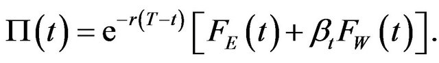
As an application to risk management in industries, we could also consider the dynamic hedging strategy of other futures by using weather future. Take the energy futures for example, if we consider a portfolio at time containing one unit of energy (e.g. heating oil) future and units of weather futures both with maturity at time T. Assume the portfolio has value at time then

If the portfolio is self-financing, the change in this portfolio in a small amount of time is given by

Assume the energy future and weather future followed by a model we have built in this paper, the future hedge ratio

In this case, the stochastic component of portfolio vanishes and the portfolio value is hedged. Thus, in order to hedge an energy future, we can short shares of weather futures and the portfolio is hedged dynamically.

Future discussion about this idea will be centered on two viewpoints. Firstly, further research need to be done for the dynamics of energy future and weather future. As such, explicit dynamic hedging conclusion regarding to hedging risks of energy commodities could be founded. The other point of view is allowing other closely related derivatives to be involved into the constructing of portfolio. For instance, we could also take the newly burgeoning carbon dioxide derivatives into account in the portfolio. These considerations will be a comprehensive tool to integrate into hedging of energy commodities’ risks.

REFERENCES

- L. Zeng, “Weather Derivatives and Weather Insurance: Concept, Application and Analysis,” Bulletin of the American Meteorological Society, Vol. 81, No. 9, 2000, pp. 2075-2081. doi:10.1175/1520-0477(2000)081<2075:WDAWIC>2.3.CO;2
- M. Cao and J. Wei, “Pricing the Weather,” Risk Magazine, May 2000, pp. 67-70.
- F. Dornier and M. Queruel, “Caution to the Wind,” Energy and Power Risk Management, 2000, pp. 30-32.
- M. H. A. Davis, “Pricing Weather Derivative by Marginal Value,” Quantitative Finance, Vol. 1, No. 3, 2001, pp. 305- 308. doi:10.1080/713665730
- D. C. Brody, J. Syroka and M. Zervos, “Dynamical Pricing of Weather Derivatives,” Quantitative Finance, Vol. 2, No. 3, 2002, pp. 189-198. doi:10.1088/1469-7688/2/3/302
- F. E. Benth, “On Arbitrage-Free Pricing of Weather Derivatives Based on Fractional Brownian Motion,” Applied Mathematical Finance, Vol. 10, No. 4, 2003, pp. 303- 324. doi:10.1080/1350486032000174628
- F. E. Benth and J. Šaltytė-Benth, “Sthochastic Modeling of Temperature Variations with a View towards Weather Derivatives,” Applied Mathematical Finance, Vol. 12, No. 1, 2005, pp. 53-85. doi:10.1080/1350486042000271638
- F. E. Benth and J. Šaltytė-Benth, “The Volatility of Temperature and Pricing of Weather Derivatives,” Quantitative Finance, Vol. 7, No. 5, 2007, pp. 553-561. doi:10.1080/14697680601155334
- F. E. Benth, J. Šaltytė-Benth and S. Koekebakker, “Putting a Price on Temperature,” Scandinavian Journal of Statistics, Vol. 34, No. 4, 2007, pp. 746-767.
- A. D. Zapranis and A. Alexandridis, “Modeling the Temperature Time-Dependent Spped of Mean Reversion in the Context of Weather Derivatives Pricing,” Applied Mathematical Finance, Vol. 15, No. 4, 2008, pp. 355-386. doi:10.1080/13504860802006065
- A. Papapantoleon, “An Introduction to Lévy Processes with Applications in Finance,” Lecture Notes, Berlin, 2008. http://page.math.tu-berlin.de/~papapan/papers/introduction.pdf
- P. Alaton, B. Djehiche and D. Stillberger, “On Modeling and Pricing Weather Derivatives,” Applied Mathematical Finance, Vol. 9, No. 8, 2002, pp. 1-20. doi:10.1080/13504860210132897
- A. J. McNeil, R. Frey and P. Embrechts, “Quantitative Risk Management: Concepts, Techniques and Tools,” Princeton University Press, Princeton, 2005.
- P. J. Brockwell and T. Marquardt, “Lévy-Driven and Fractionally Integrated ARMA Processes with Continuous Time Parameter,” Statistica Sinica, Vol. 15, No. 2, 2005, pp. 477-494.
- F. E. Benth, J. Šaltytė-Benth and S. Koekebakker, “Stochastic Modeling of Electricity and Related Markets,” World Scientific Press, The Singapore City, 2008.
- F. E. Benth and J. Šaltytė-Benth, “The Normal Inverse Gaussian Distribution and Spot Price Modeling in Energy Markets,” International Journal of Theoretical Applied Finance, Vol. 7, No. 2, 2004, pp. 177-192. doi:10.1142/S0219024904002360
- E. Hewitt and K. R. Stromberg, “Real and Abstract Analysis: A Modern Treatment of the Theory of Functions of a Real Variable,” Springer-Verlag, Berlin, 1965.
- K. Chourdakis, “Option Pricing Using the Fractional FFT,” Journal of Computational Finance, Vol. 8, No. 2, 2004, pp. 1-18.