Open Journal of Statistics
Vol. 3 No. 5 (2013) , Article ID: 37654 , 12 pages DOI:10.4236/ojs.2013.35040
Aggregating Density Estimators: An Empirical Study
1Instituto de Matemática y Estadística, Facultad de Ingeniería, Universidad de la República, Montevideo, Uruguay
2Institut de Mathématiques de Luminy, Université d’Aix-Marseille, Marseille, France
Email: mbourel@fing.edu.uy, badih.ghattas@univ-amu.fr
Copyright © 2013 Mathias Bourel, Badih Ghattas. This is an open access article distributed under the Creative Commons Attribution License, which permits unrestricted use, distribution, and reproduction in any medium, provided the original work is properly cited.
Received June 20, 2013; revised July 20, 2013; accepted July 27, 2013
Keywords: Machine Learning; Histogram; Kernel Density Estimator; Bagging; Boosting; Stacking
ABSTRACT
Density estimation methods based on aggregating several estimators are described and compared over several simulation models. We show that aggregation gives rise in general to better estimators than simple methods like histograms or kernel density estimators. We suggest three new simple algorithms which aggregate histograms and compare very well to all the existing methods.
1. Introduction
Ensemble learning or aggregation methods are among the most challenging recent approaches in statistical learning. In a supervised framework, the main goal is to estimate a function  using a data set of independent observations of both variables
  and
and  Ensemble learning constructs several such estimates
 , which are often called weak learners, and combines them to obtain the aggregated model
  where
where  may be a simple or a weighted average when
  such as for regression, or a simple or a weighted majority voting rule when
  such as for classification. In this framework, Bagging ([1]), Boosting ([2]), Stacking ([3]), and Random Forests ([4]) have been declared to be the best of the shelf classifiers achieving very high performances when tested over tens of various datasets selected from the machine learning benchmark. All these algorithms had been designed for supervised learning, and sometimes initially restricted to regression or binary classification. Several extensions are still under study: multivariate regression, multiclass learning, and adaptation to functional data or time series.
Very few developments exist for ensemble learning in the unsupervised framework, clustering analysis and density estimation. Our work concerns the latter case which may be seen as a fundamental problem in statistics. Among the latest developments, we found some extensions of Boosting ([2]) and Stacking ([5]) to density estimation. The existing methods seem to be quite complex, often combining kernel density estimators and whose parameters seem to be arbitrary. In particular, most of the methods combine a fixed number of weak learners.
In this paper we show extensive simulations that aggregation gives rise to effective better estimates than simple classical density estimators. We suggest three simple algorithms for density estimation in the same spirit of bagging and stacking, where the weak learners are histograms. We compare our algorithms to several algorithms for density estimation, some of them are simple like Histogram and Kernel Density Estimators (Kde) and others rather complex like stacking and boosting, which will be described in details. As we will show in the experiments, although the accuracy of our algorithms is not systematically higher than other ensemble methods, they are simpler, more intuitive and computationally less expensive. Up to our knowledge, the existing algorithms have never been compared over a common benchmark simulation data.
Aggregating methods for density estimation are described in Section 2. Section 3 describes our algorithms. Simulations and results are given in Section 4 and concluding remarks and future work are described in Section 5.
2. A Review of the Existing Algorithms
In this Section we review some density estimators obtained by aggregation. They may be classified in two categories depending on the aggregation form.
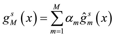
The first type has the form of linear or convex combination:
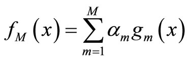 (1)
(1)
where  and
and  is typically a parametric or non parametric density model, and in general different values of m refer typically to different parameters values in the parametric case or different kernels or different bandwidths for a chosen kernel for the kernel density estimators.
The second type of aggregation is multiplicative and is based on the ideas of high order bias reduction for kernel density estimation as in [6]. The aggregated density estimator has the form:
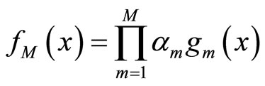 (2)
(2)
2.1. Linear or Convex Combination of Density Estimators
This kind of estimators (1) has been used in several works with different construction schemes.
• In [7-9] the weak learners  are introduced sequentially in the combination. At step m,
  is a density selected among a fixed class H and is chosen to maximize the log likelihood of
 (3)
(3)
In [8],  is selected among a non parametric family of estimators, and in [7,9], it is taken to be a Gaussian density or a mixture of Gaussian densities whose parameters are estimated. Different methods are used to estimate both density
  and the mixture coefficient
 .
.
In [7],  is a Gaussian density and the log likelihood of (3) is maximized using a special version of Expectation Maximization (EM) taking into account that a part of the mixture is known.
The main idea underlying the algorithms given by [8,9] is to use Taylor expansion around the negative log likelihood that we wish to minimize:
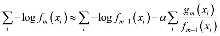
where  is the data set. Thus, minimizing the left side term is equivalent to maximizing
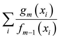 , and the output of this method converges to a global minimum.
All the algorithms described above are sequential and the number of weak learners aggregated may be fixed by the user.
• In [5], Smith and Wolpert used stacked density estimator applying the same aggregation scheme as in stacked regression and classification ([10]). The M densities estimators  are fixed in advance (KDE with different bandwidths). The data set
  is divided into V cross validation subsets
 . For
. For , denote
 .
.
The M models  are fitted using the training samples
  and the obtained estimates are denoted by for all
  These models are then evaluated over the test samples
  getting the vectors
  for
for  put within a
  block matrix:
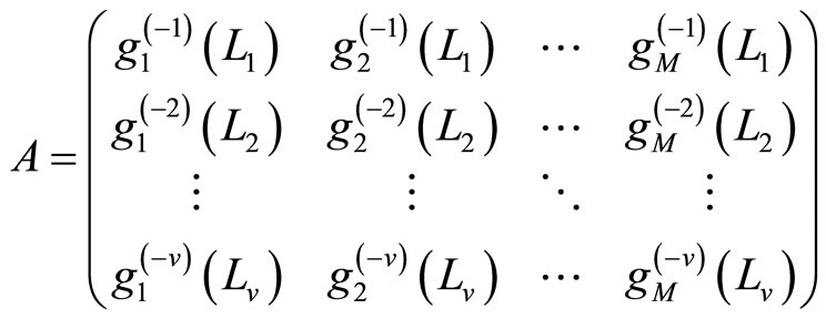
This matrix is used to compute the coefficients 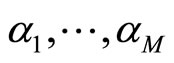 of the aggregated model (1) using the EM algorithm. Finally, for the output model, we re-estimate the individual densities
  from the whole data.
This method has been compared with other algorithms including the best single model obtained by cross-validation, the best single model obtained over a test sample and a uniform average of the different Kde models. It is shown that stacking outperforms these methods for different criteria: log likelihood, L1 and L2 performance measures (for the two last criteria use the true density).
• In [11], Rigollet and Tsybakov fixed the densities  in advance like for stacking (Kde estimators with different bandwidths). The dataset is split in two parts. The first sample is used to estimate the densities
 , whereas the coefficients
  are optimized using the second sample. The splitting process is repeated and the aggregated estimators for each data split are averaged. The final model has the form
 (4)
(4)
where S is the set of all the splits used and
 (5)
(5)
is the aggregated estimator obtained from one split s of the data,  is the individual kernel density function estimated over the learning sample obtained from the split s. This algorithm is called AggPure. The authors compared their algorithm using different choices for the Kde’s bandwidth that we describe in the simulations section. Oracle inequalities and risk bounds are given for this estimator.
2.2. Multiplicative Aggregation
The only algorithm giving rise to this form of aggregation is the one described in [12] called BoostKde. It is a sequential algorithm where at each step m the weak learner is computed as follows:
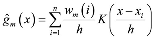 (6)
(6)
where K is a fixed kernel, h its bandwidth, and 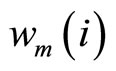 the weight of observation i at step m. Like for boosting, the weight of each observation is updated by
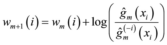 (7)
(7)
where 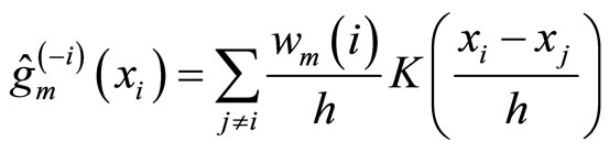
The output is given by
 (8)
(8)
where C is a normalization constant.
Using several simulation models the authors explore different values for the bandwidth h minimizing the Mean integrated Square Error (MISE) for few values of M. They show that a bias reduction is obtained for M = 2 but it is not clear how the algorithm behaves for more than two steps.
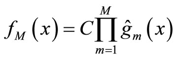
3. Aggregating Histograms
We suggest three new density estimators obtained by linear combination like in (1), all of them use histograms as weak learners. The first two algorithms aggregate randomized histograms and may be parallelized. The third one is just an adaptation of Stacking using histograms instead of kernel density estimators.
The first algorithm is similar to Bagging ([1]). Given a data set  and an integer L, at each step
 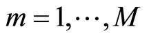 of the algorithm a bootstrap sample of T is generated and used to construct an histogram
  with L equally spaced breakpoints. The output of this method is an average of the M histograms. We will refer to this algorithm as BagHist and it is detailed in Figure 1.
The second algorithm, AggregHist, works as follows. Consider the data set  and an integer L.
Figure 1. Bagging histograms (BagHist).
Let  be the histogram obtained over T using equally spaced breakpoints denoted by
 . We denote by
  for all
  the bandwidth of
 . At each step
  we add a random uniform noise
  to each breakpoint and construct an histogram
  using T and the new set of breakpoints. The final output is an average of the histograms
 . The algorithm is detailed in Figure 2.
The value of the parameter L used for AggregHist and BagHist will be optimized and the procedure used for that will be described in the next Section.
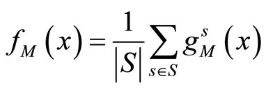
Finally, we introduce a third algorithm called StackHist where we replace in the stacking algorithm the six kernel density estimators by histograms with different number of breakpoints.
4. Experiments
In this Section we present the simulations we have done to compare all the methods described in Section 2 together with our three algorithms. We consider several data generating models we have found in the literature. We first show how our algorithms adjust quite well for the different models, and that the adjustment error decreases monotonically with the numbers of histograms used. Finally we will compare our methods with ensemble methods for density estimation like Stacking, AggPure, BoostKde which aggregated non parametric density estimators. All these aggregating methods are compared to optimized Histogram (Hist) and Kde using different bandwidth optimization approaches.
4.1. Models Used for the Simulations
Twelve models found in the papers we have referenced are used in our simulations. We denote them by M1,···, M12 and we group them according to their difficulty level.
• Some standard densities used in [11,12]:
(M1) standard Gaussian density ,
,
(M2) standard exponential density,
(M3) a Chisquare density ,
,
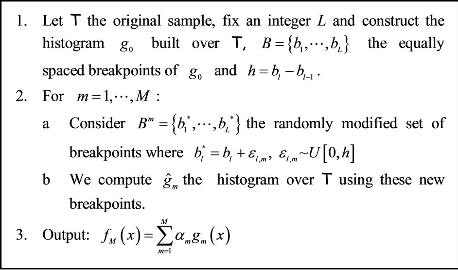
Figure 2. Aggregating histograms based on randomly perturbed breakpoints (AggregHist).
(M4) a student density t4,
• Some Gaussian mixtures taken from [5,12]:
(M5) ,
,
(M6) 
(M7) 
• Gaussian mixtures used in [11] and taken from [13]:
(M8) the Claw density,
(M9) the Smooth Comb density,
• (M10) is a mixture density with highly inhomogeneous smoothness as in [12]
• Finally we include in our study two simple models known to be challenging for density estimators:
(M11) a triangular density with support [0,1] and maximum at 1,
(M12) the beta density with parameters 2 and 5.
All the simulations are done with the R software, and for models M8 and M9 we use the benchden package. Figure 3 shows the shape of the densities we have used to generate the data sets.
Figure 4 shows, for some models, the estimator obtained using AggregHist (red curve), BagHist (green curve)
and StackHist (blue curve) for n = 1000 observations and M = 150 histograms for the two first algorithms. A simple histogram is shown together with the three estimates. For StackHist we aggregate six histograms having 5, 10, 20, 30, 40 and 50 equally spaced breakpoints and a ten fold cross validation is used. Both AggregHist and BagHist give more smooth estimators than StackHist.
Figures 5 and 6 show the adjusted densities obtained from AggregHist and BagHist when increasing the number M of histograms for model M7.
4.2. Tuning the Algorithms
We compare the following algorithms AggregHist, BagHist, StackHist, Stacking, AggPure and BoostKde with some classical methods like Hist and Kde.
For AggregHist and BagHist we fix the number of histograms to M = 200. The number of breakpoints is optimized testing different values over a fixed grid of 10, 20 and 50 equally spaced breakpoints. The optimal value retained for each model is the one which maximizes the log likelihood over 100 independent test samples drawn
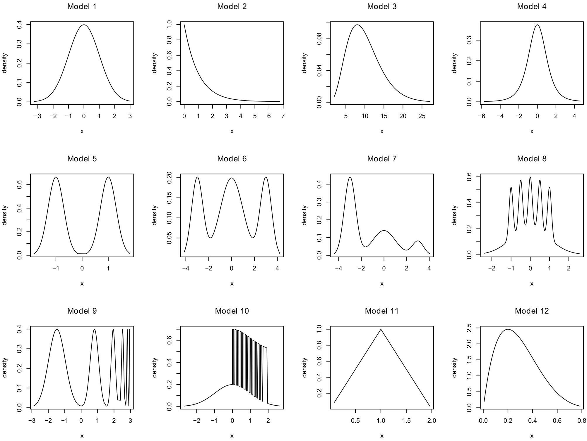
Figure 3. Densities used for the simulations.
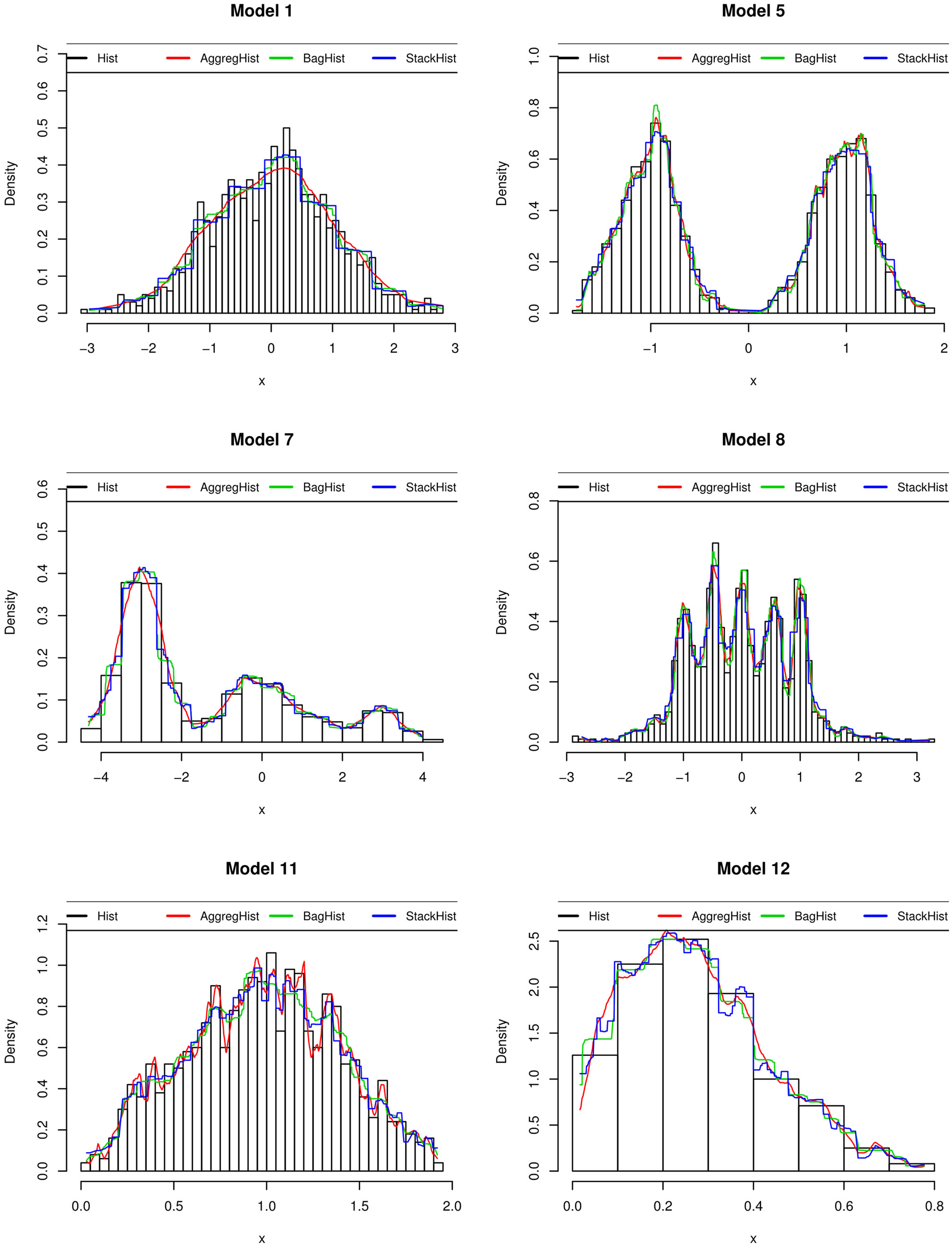
Figure 4. Density estimators obtained used for Hist, AggregHist (red curve), BagHist (green curve) and StackHist (blue curve) for 6 models among those used in the simulations.
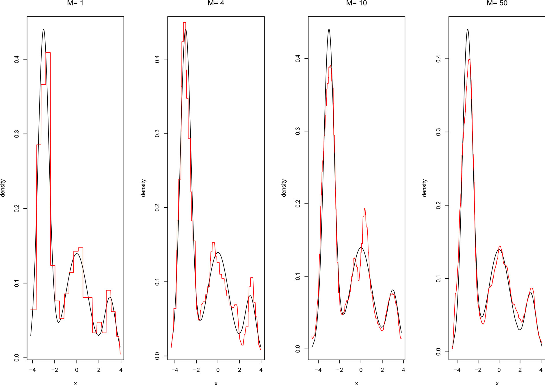
Figure 5. Density estimate given by AggregHist with different values of M for model M7.
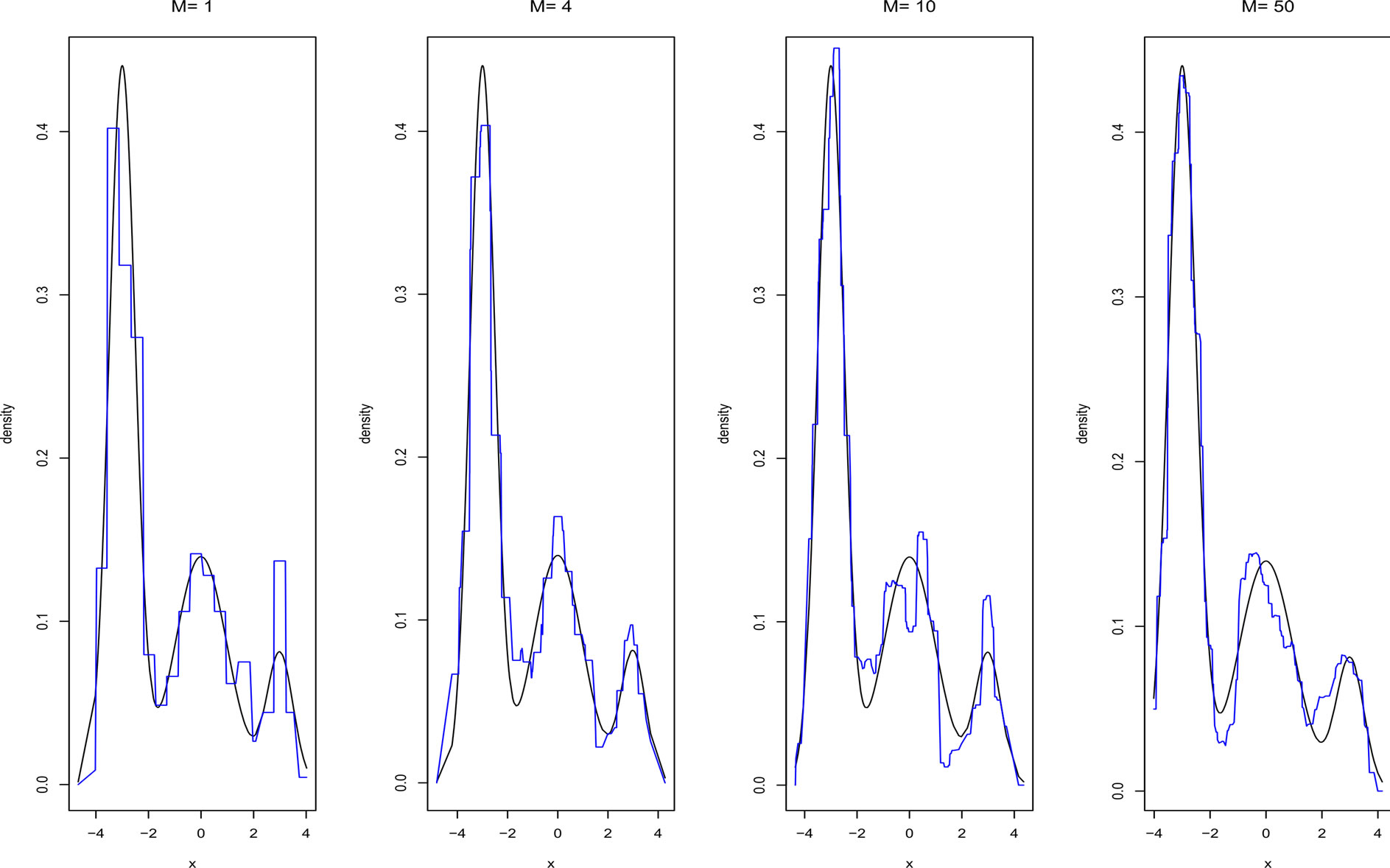
Figure 6. Density estimate given by BagHist with different values of M for model M7.
from the corresponding model. We optimize the number of breakpoints of the histogram in the same way as for our algorithms. These optimal values are given in Table 1 for differents values of n (100, 500 and 1000). We denote the optimal number of breakpoints LH, LBH and LAH for Hist, BagHist and AggregHist respectively.
To make the comparisons as faithful as possible, we have used for the other methods the same values suggested by their corresponding authors:
• For Stacking, six kernel density estimators are aggregated, three of them use Gaussian kernels with fixed bandwidths h = 0.1, 0.2, 0.3 and the others use traingular kernels with bandwidths h = 0.1, 0.2, 0.3. The number of cross validation samples is V = 10.
• For AggPure six kernel density estimators are aggregated having bandwidths 0.001, 0.005, 0.01, 0.05, 0.1 and 0.5. Instead of the quadratic algorithm used by the authors in [11], we optimize the coefficients of the linear combination with the EM algorithm. The final estimator is a mean over |S| = 10 random splits of the original data set.
• For BoostKde, we use 5 steps for the algorithm aggregating kernel density estimators whose bandwidths are optimized using Silverman rule of thumbs (see Appendix). Normalization of the output is done using numerical integration. Extensive simulations we have done using BoostKde showed that more steps give rise to less accurate estimators and unstable results.
For Kde we use a standard gaussian kernel and some common data driven bandwidth selectors:
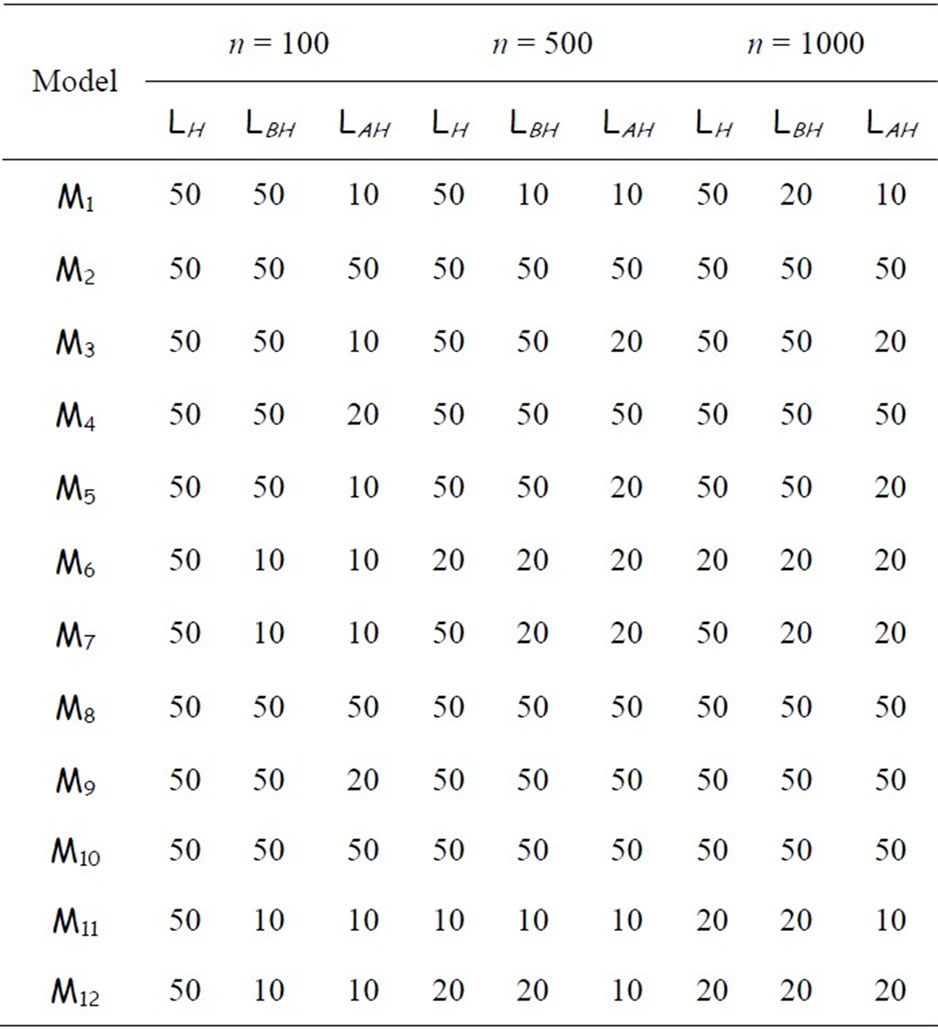
Table 1. Optimal number of breakpoints used for Hist and our algorithms for each model and for each value of n.
• the Silverman’s rules of thumb ([14]) using factor 1.06 (KdeNrd) and factor 0.9 (KdeNrd0),
• the unbiased cross-validation rule (KdeUCV, [15]),
• the Sheater Johns plug-in method (KdeSJ, [16,17]).
These choices are described in details in the appendix.
4.3. Results
The performance of each estimator is evaluated using the Mean Integrated Squared Error (MISE):
 (9)
(9)
where  is the true density and
  its estimate. It is computed as the average of the integrated squared error
 (10)
(10)
over 100 Monte Carlo simulations.
For the same simulations, we have also computed the log likelihood criterion whose maximization is equivalent to reducing the Kullback-Leibler divergence between the true and the estimated densities (see P. Hall, “On Kullback-Leibler loss and density estimation”, Ann. Stat., Vol. 15, 1987). The results obtained using this criterion are unstable due to numerical approximation of the log likelihood for small values of the densities. In particular the histogram has very good performance with respect to the log likelihood when compared to all the other methods. This is due to the fact that when computing the log likelihood we omit the points i for which  equals zero, and such points appear much more for the histogram than for the other methods. For all these reasons we do not report these results.
Figure 7 shows how the MISE varies when increasing the number of histograms in AggregHist and BagHist. For all the models, the adjustment error decreases significantly for the first 100 iterations. In most of the cases AggregHist gives a better estimate than BagHist.
Table 2 shows the execution time for AggregHist, BagHist, Stacking and AggPure for n = 2000. The other algorithms need much less time as they combine very few simple estimators and do not use any resampling. Computing time is significantly lower for our algorithms.
We compare now all the algorithms cited above over the twelve models using n = 100, n = 500 and n = 1000. For AggregHist and BagHist we use M = 200 histograms. Tables 3 to 5 summarize the results for each value of n = 100, 500 and 1000. For each model and each method we give the average of 100 × MISE over 100 Monte Carlo simulations. For the Kde we kept the best result among the four choices of bandwidth selectors (nrd, nrd0, ucv and sj), the best choice being between brackets. The best result for each simulation model is put in bold.
It is clear that no method outperforms all the others in all the cases and for all the methods the error decreases
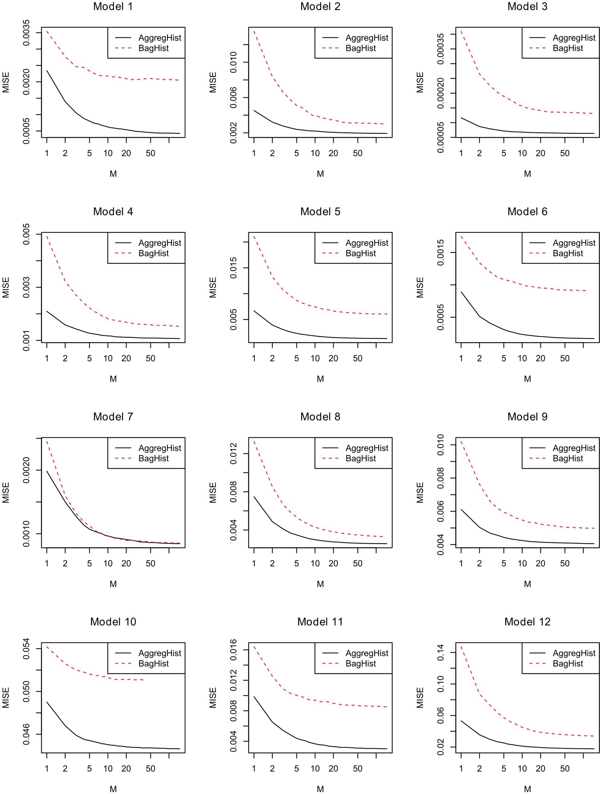
Figure 7. MISE error versus number of aggregated histograms in AggregHist and BagHist for models 1 to 12.
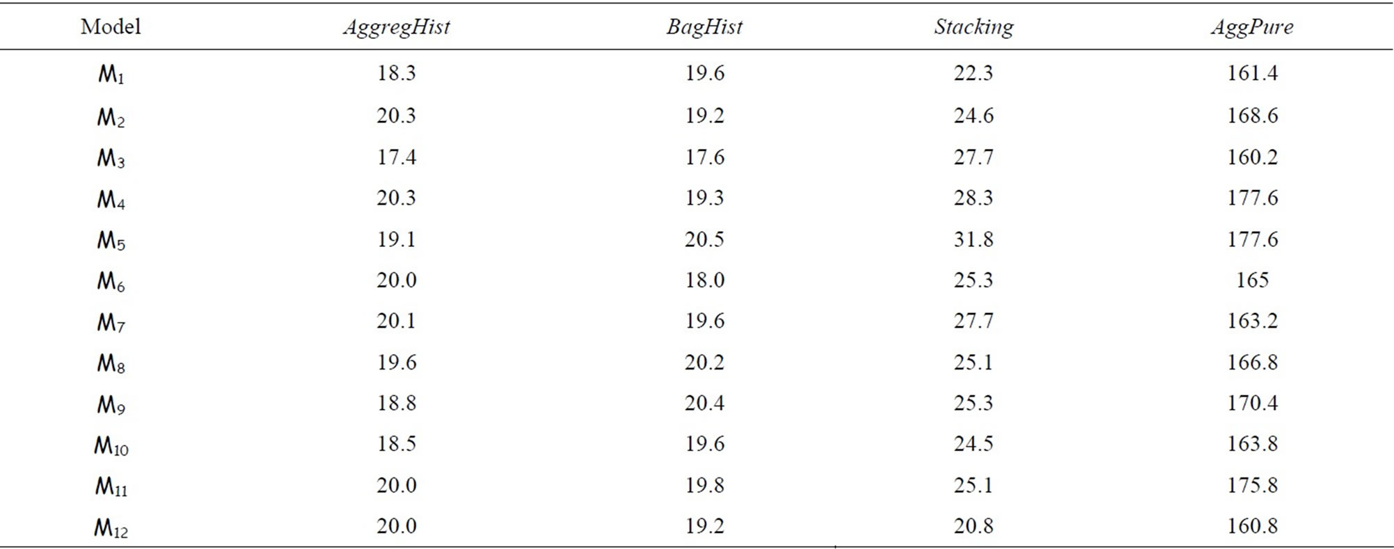
Table 2. Time (in seconds) elapsed for each model for AggregHist, BagHist, Stacking and AggPure taking n = 2000 and M = 50.
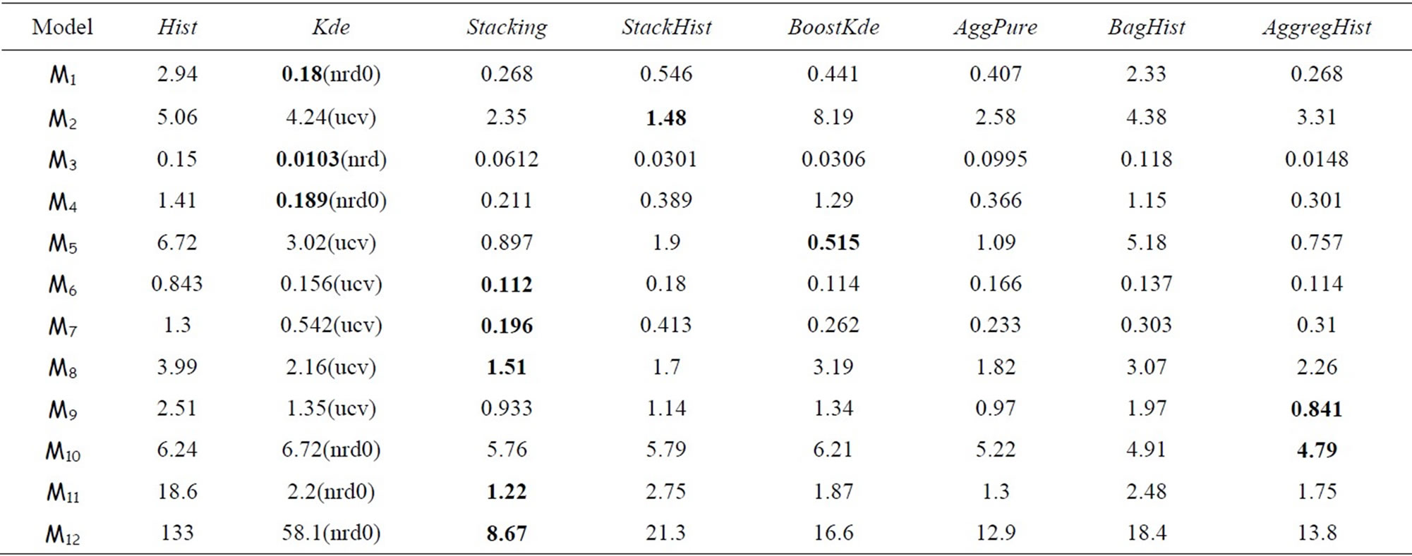
Table 3. 100 × MISE with n = 100 and M = 200.
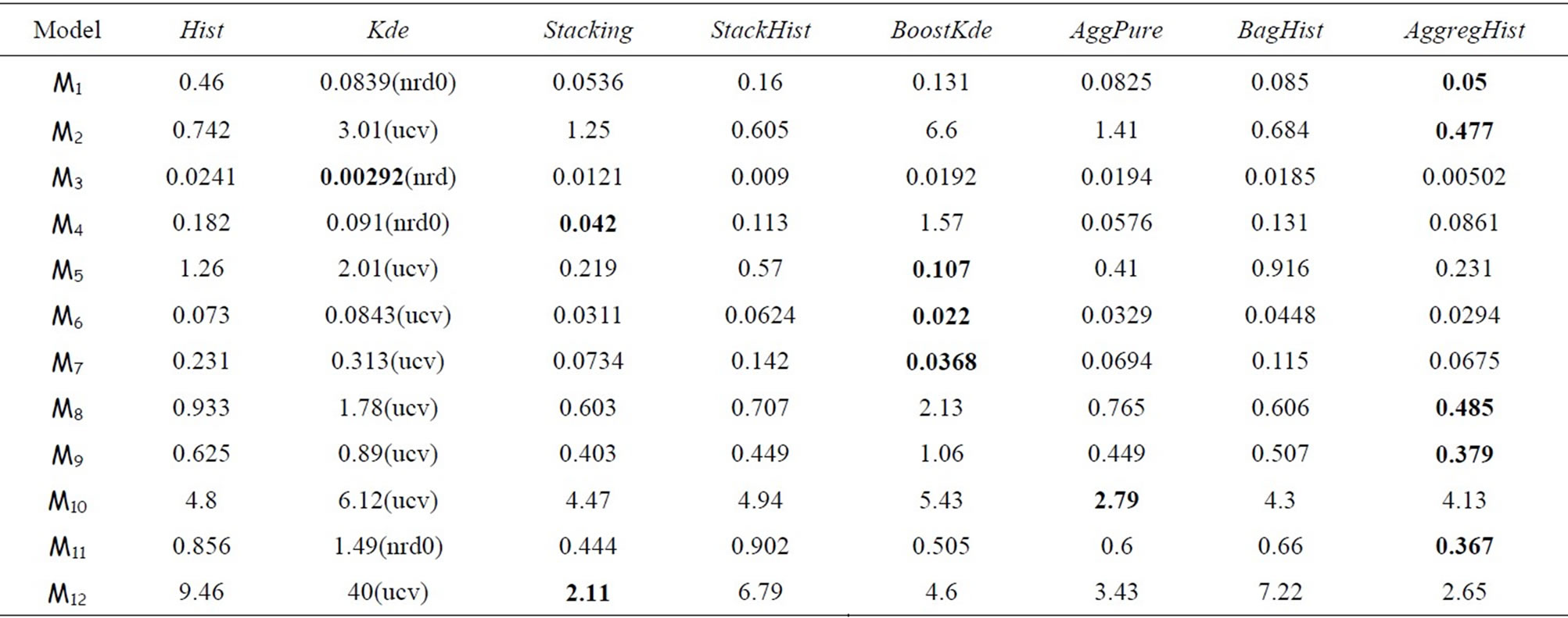
Table 4. 100 × MISE with n = 500 and M = 200.
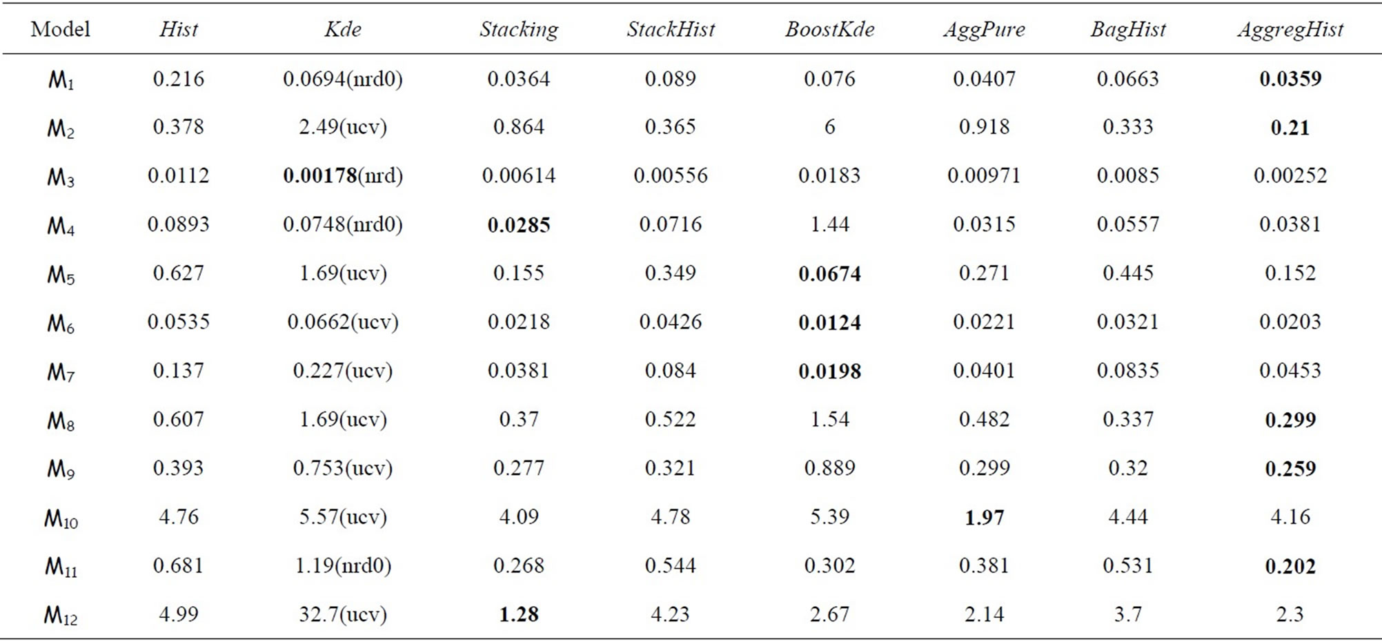
Table 5. 100 × MISE with n = 1000 and M = 200.
when increasing the sample size. Ensemble methods estimators outperform largely the Hist and Kde in most cases except three models (standard gaussian,  and student distributions) for n = 100, and only the
  model for n = 500 and 1000. For the gaussian mixtures models BoostKde gives the best results for the largest values of n (500 and 1000). Stacking outperforms the other algorithms for the student and the triangular distributions for n = 1000. For model M10, AggPure achieves the best performance. For the remaining simulation models, AggregHist outperforms all the other methods when n = 1000. When it is doesn’t achieve the lowest error, it is still very close to the best especially for the most challenging distributions used in models M8 to M12.
5. Conclusion
In this paper we have given a brief summary of most existing approaches for density estimation based on aggregation. We have shown using a wide range of simulations that, like for supervised learning, ensemble methods give rise to better density estimators than the Histogram and the Kernel Density Estimators. Among the existing methods we have tested direct extensions of stacking (Stacking) and of boosting (BoostKde) as well as the most recent approach found in the literature called AggPure.
We have also suggested three new algorithms among which two of them BagHist and AggregHist combine a large number of histograms. BagHist randomizes the data using bootstrap samples whereas AggregHist uses the original data set, randomizing the histogram breakpoints. AggregHist gives very good results for most of the situations especially for large sample sizes, and it is easy to implement and has the lowest computation cost among all the ensemble density estimators.
Most of the presented algorithms may be extended to the multivariate case and are now under study both empirically and theoretically. All the simulations and the methods have been implemented within an R package available upon request.
6. Acknowledgements
The authors would like to thank Claude Deniau and Ricardo Fraiman for many useful discussions and suggestions that have improved this work.
REFERENCES
- L. Breiman, “Bagging Predictors,” Machine Learning, Vol. 24, No. 2, 1996, pp. 123-140. http://dx.doi.org/10.1007/BF00058655
- Y. Freund and R. E. Schapire, “A Decision-Theoretic Generalization of On-Line Learning and Application to Boosting,” Journal of Computer and System Sciences, Vol. 55, No. 1, 1997, pp. 119-139. http://dx.doi.org/10.1006/jcss.1997.1504
- L. Breiman, “Stacked Regression,” Machine Learning, Vol. 24, No. 1, 1996, pp. 49-64.
- L. Breiman, “Random Forests,” Machine Learning, Vol. 45, No. 1, 2001, pp. 5-32. http://dx.doi.org/10.1023/A:1010933404324
- P. Smyth and D. H. Wolpert, “Linearly Combining Density Estimators via Stacking,” Machine Learning, Vol. 36, No. 1, pp. 59-83.
- M. Jones, O. Linton and J. Nielsen, “A Simple Bias Reduction Method for Density Estimation,” Biometrika, Vol. 82, No. 2, 1995, pp. 327-338. http://dx.doi.org/10.1093/biomet/82.2.327
- G. Ridgeway, “Looking for Lumps: Boosting and Bagging for Density Estimation,” Computational Statistics & Data Analysis, Vol. 38, No. 4, 2002, pp. 379-392. http://dx.doi.org/10.1016/S0167-9473(01)00066-4
- S. Rosset and E. Segal, “Boosting Density Estimation,” Advances in Neural Information Processing Systems, Vol. 15, MIT Press, 2002, pp. 641-648.
- X. Song, K. Yang and M. Pavel, “Density Boosting for Gaussian Mixtures,” Neural Information Processing, Vol. 3316, 2004, pp. 508-515. http://dx.doi.org/10.1007/978-3-540-30499-9_78
- D. H. Wolpert, “Stacked Generalization,” Neural Networks, Vol. 5, No. 2, 1992, pp. 241-259. http://dx.doi.org/10.1016/S0893-6080(05)80023-1
- P. Rigollet and A. B. Tsybakov, “Linear and Convex Aggregation of Density Estimators,” Mathematical Methods of Statistics, Vo. 16, No. 3, 2007, pp. 260-280. http://dx.doi.org/10.3103/S1066530707030052
- M. Di Marzio and C. C. Taylor, “Boosting Kernel Density Estimates: A Bias Reduction Technique?” Biometrika, Vol. 91, No. 1, 2004, pp. 226-233. http://dx.doi.org/10.1093/biomet/91.1.226
- J. S. Marron and M. P. Wand, “Exact Mean Integrated Square Error,” The Annals of Statistics, Vol. 20, No. 2, 2004, pp. 712-736. http://dx.doi.org/10.1214/aos/1176348653
- B. W. Silverman, “Density Estimation for Statistics and Data Analysis,” Chapman and Hall, London, 1986.
- A. Bowman, “An Alternative Method of Cross-Validation for the Smoothing of Density Estimates,” Biometrika, Vol. 71, No. 2, 1984 pp. 353-360. http://dx.doi.org/10.1093/biomet/71.2.353
- S. J. Sheather, “Density Estimation,” Statistical Science, Vol. 19, No. 4, 2004, pp. 588-597. http://dx.doi.org/10.1214/088342304000000297
- W. Härdle, M. Müller, S. Sperlich and A. Werwatz, “Nonparametric and Semiparametric Models,” Springer Verlag, Heidelberg, 2004. http://dx.doi.org/10.1007/978-3-642-17146-8
- S. J. Sheather and M. C. Jones, “A Reliable Data-Based Bandwidth Selection Method for Density Estimation,” Journal of the Royal Statistical Society, Vol. 53, No. 3, 1991, pp. 683-690.
Appendix
Different Choices for the Bandwidth Selection in KDE
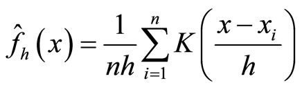
If 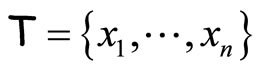 denotes a sample obtained from a random variable X with density f, the kernel density estimation of f at point x is:
 (11)
(11)
where K is a kernel function.
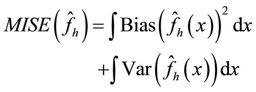
A usual measure of the difference of the estimate density and the true density is the Mean integrated Squared Error (MISE) which may be written as:
 (12)
(12)
It is well known
with  and
and  where
where 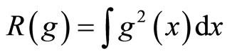
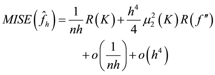
and 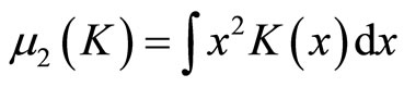 The Asymptotic Mean Integrated Squared Error (AMISE) is:
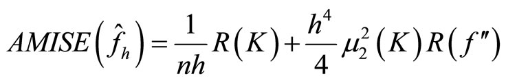 (13)
(13)
and it is minimized for
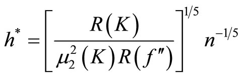 (14)
(14)
Taking Gaussian kernel K and assuming that the underlying distribution is normal, Silverman ([14]) showed that the expression of  is
is
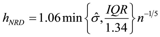 (15)
(15)
where  and IQR are the standard deviation and the interquantile distance respectively of the sample. This is known as Silverman’s rule of thumbs. Furthermore Silverman recommended to use for the constant the values 0.9 (Nrd0) or 1.06 (Nrd).
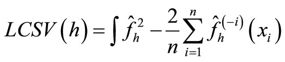
Another choice of the bandwidth is given by the cross validation method ([15]). Here we consider the Integrated squared error (ISE) which is given by
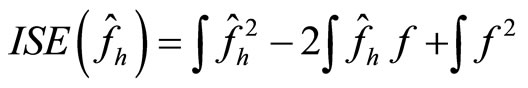 (16)
(16)
Observe that the last term does not involve h. The least squares cross-validation is
 (17)
(17)
where  denotes the kernel estimator constructed from the data without the observation i. In [17], it is proved rewriting
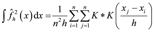 (18)
(18)
where * denotes the convolution, that 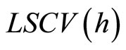 is an
is an
estimator of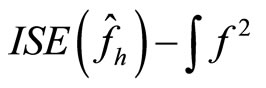 . Moreover it is easy to verify that
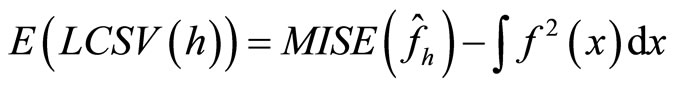 , thus the
least squares cross-validation is also called unbiased crossvalidation. We denote by  the value of h which minimizes
 .
.
Finally, the plug-in method of Sheather and Jones replaces the unknown  used in the optimal value of
h by an estimator  where g is a “pilot bandwidth”
which depends on h (see [16-18] for more details).