Open Journal of Statistics
Vol.2 No.5(2012), Article ID:25548,8 pages DOI:10.4236/ojs.2012.25065
Bayesian Factorized Cointegration Analysis
1Department of Statistical Science, Duke University, Durham, USA
2School of Science and Information, Qingdao Agricultural University, Qingdao, China
Email: kc52@stat.duke.edu, wshcui@qau.edu.cn
Received October 25, 2012; revised November 30, 2012; accepted December 8, 2012
Keywords: Cointegration; Bayesian; Dynamic Factor; Non-Stationary; Root Structure; MCMC
ABSTRACT
The concept of cointegration is widely used in applied non-stationary time series analysis to describe the co-movement of data measured over time. In this paper, we proposed a Bayesian model for cointegration test and analysis, based on the dynamic latent factor framework. Efficient computational algorithms are also developed based on Markov Chain Monte Carlo (MCMC). Performance and efficiency of the the model and approaches are assessed by simulated and real data analysis.
1. Introduction
Many macroeconomic and financial time series are nonstationary [1], characterized by the existence of stochastic trends or unit roots. Thus, modeling multivariate nonstationary time series via linear regression, while has been widely used on stationary time series analysis, has been shown to be a dangerous approach that could produce spurious regression [1]. Alternatively, if linear combinations of non-stationary or unit-root variables are stationary, then cointegration is said to occur, which is often observed in practice. Since the development of the concept of cointegration [2], there has been a rich literature on testing cointegration and inference using such models. However, most of the work adopted a classical econometric perspective based on the linear cointegrated error correction models. In this study, the Bayesian factorized cointegration analysis proposed here as a different perspective shed new lights on many key properties of cointegration models.
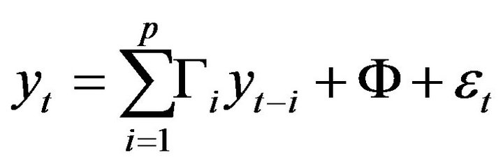
To establish the notion and illustrate the basic ideas underlying classical cointegration analysis, let ![]() be a realization of Q dimensional Vector Autoregressive (VAR) process of lag order p:
be a realization of Q dimensional Vector Autoregressive (VAR) process of lag order p:
where .
.  denotes the autoregression intercept. This model can be written in the Vector Error Correction Model (VECM) form as:
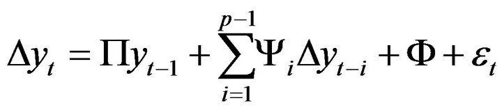
where the matrix  of rank r can be written as
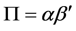 , where
 ![]() and
and  are both full rank
  matrices, with
  denoting the number of cointegration relationships. Note that as a special case, when
  is zeros matrix with
 , then all time series are non-stationary with unit roots, but no cointegration relationship exists.
  is called the cointegration vector with
  being stationary.
Classical cointegration tests have been developed based on the VECM models to test the rank of . For example, Johansen test [3] is considered as a generally applicable test for multivariate non-stationary time series that allows more than one cointegration relationship. While in practice when cointegration is often used for two time series, the Engle-Granger two-step method [2] has also been widely used. However, all the classical methods have their clear limitations when applied in practice. Johansen method, as a more general cointegration test method than the other two, is a complicated model with many degrees of freedom. Also, it has to model all the variables at the same time without a clear and straightforward interpretation in terms of exogenous and endogenous variables, which are all less favorable with multivariate cases especially if the relation for some variable is flawed. On the other hand, as the most wellknown test for cointegration of two time series, the Engle-Granger test simply tests the stationarity of a given linear combination of two time series based on unit root tests (e.g. ADF test), where the cointegration ratio is obtain by running a static regression of the two time series. However, the two-step procedure suffers from many problems (e.g. multiple testing) and fails in many cases to be an effective approach to identify cointegrated pairs in practice.
In this paper, we propose the framework of Bayesian factorized cointegration analysis as a straightforward and computationally efficient approach for cointegration test and modeling. Although the dynamic latent factor model has been proposed for time series analysis for decades, the idea of incorporation of dynamic structures that can accommodate possible non-stationarity flexibly enough via the Bayesian modeling framework and computational strategies, which we proposed as an alternative Bayesian cointegration test, is novel. The model and approaches are described in in Section 2, followed by Bayesian computation and posterior analysis via Markov Chain Monte Carlo (MCMC) methods in Section 3. Section 4 applies the model to simulated data sets to gauge the performance of the models. In Section 5 the model is applied to detecting and analyzing cointegration between real nonstationary time series, with conclusions and future directions in Section 6.
2. Model Specification
2.1. Basic Dynamic Latent Factor Models
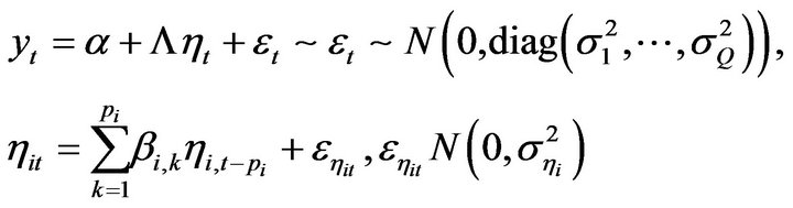
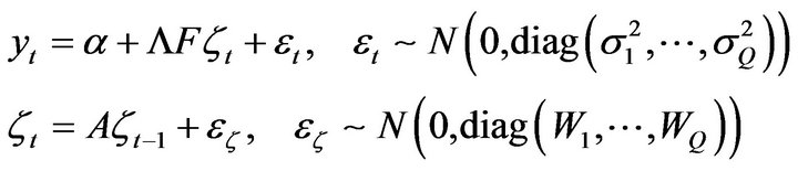
Let ![]() be a realization of Q dimensional nonstationary time series, we propose a Bayesian dynamic latent factor model to jointly model the multivariate nonstationary time series and detecting cointegration among the component time series via
be a realization of Q dimensional nonstationary time series, we propose a Bayesian dynamic latent factor model to jointly model the multivariate nonstationary time series and detecting cointegration among the component time series via  common dynamic latent factors. Specifically, let
denote the vector of q dynamic latent factors, the model is of the form:
 (1)
(1)
where  is a lower triangular factor loading matrix. Each factor
  is modeled as following a
  process that can be either stationary or non-stationary.
2.2. Model in the Matrix State-Space Form
Let ,
,
 ,
,  , where
![]() is a
is a  vector, and
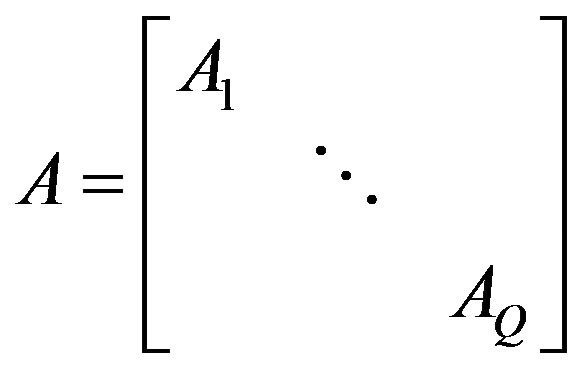 , where
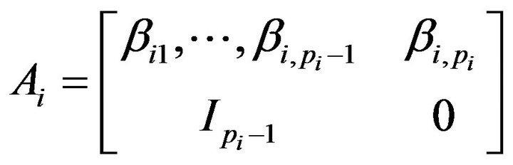 .
.
 is the transition matrix giving
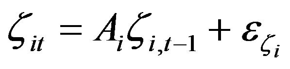 with
with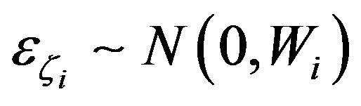 , where
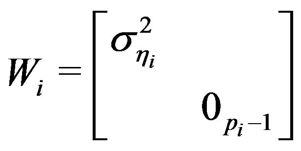 . Then model (1) can be written in the matrix state-space form:
 (2)
(2)
The matrix state-space form model (2) is primarily used in deriving efficient computational strategies for sampling latent factors as shown in the following section. As stated previously, although this dynamic latent factor model has been applied for time series analysis for decades, our idea of the incorporation of dynamic structures that can accommodate possible non-stationarity flexibly enough via the Bayesian modeling framework and computational strategies, which we proposed as an alternative Bayesian cointegration test, is novel and shown in the following sections.
2.3. Modeling Dynamic Latent Factors
The key idea of modeling multivariate nonstationary time series via independent latent factors requires flexible modeling of the dynamic factors. It is critical that the model is flexible in terms of two aspects. The values of  coefficients of the dynamic structure of latent factors need to be able to flexibly model stationary and non-stationary (unit-root) processes. And secondly, the autoregressive order p should also be flexibly modeled.
To achieve these, we followed the  process decomposition proposed by [4], with spike-and-slab priors placed on the root structures. Induced priors on the
  coefficients can be deduced. We further used half-cauchy prior for the innovation variances, as recommenced by [5] for hierarchical modeling.
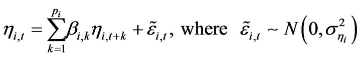
In details: given that the  time-varying latent factor is modeled via an autoregressive process with (maximum) lag order
 , we have that:
 (3)
(3)
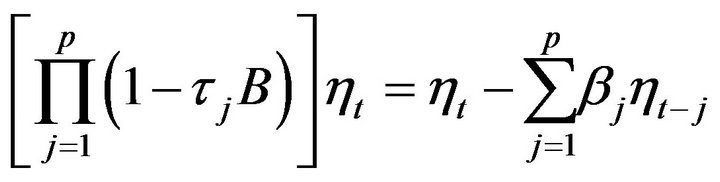
where B is the backshift operator, 
is the characteristic polynomial of the model,
 is a
is a  vector of the autoregression coefficients of the
  dynamic latent factor, and
  is white noise.
Assume that the characteristic polynomial  has
has  non-zeros real roots and
  pairs of non-zero conjugate complex roots (with
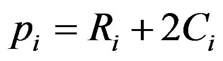 )1, then the autoregressive process can be characterized in term so either the autoregressive coefficients
  or the
 ![]() characteristic roots. Let
characteristic roots. Let 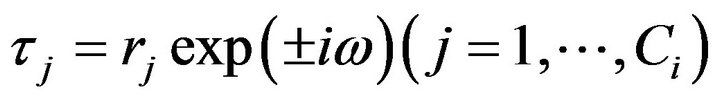 denote the
  pairs of complex roots and
 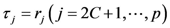 denote the real roots, then we place a class of hierarchical models on the root structures as introduced by [6], which indirectly induce models on the
  s that either fall into the stationary or unit-root process space. Specifically, the models we used are:
1) For the complex roots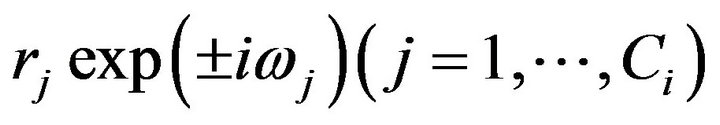 , we model the modulus
 ![]() and period
and period 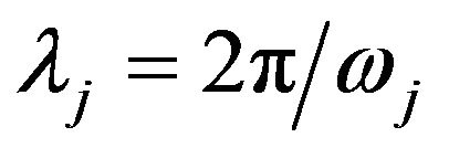 as follows:
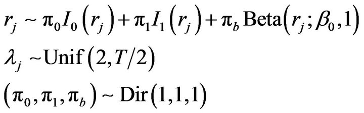 (4)
(4)
where  and
and  are Dirac delta functions at 0 and 1 respectively.
  are weights with Dirichlet prior distributions, and
 ![]() is the number of time points.
is the number of time points.
2) For the real roots, similarly we have
 (5)
(5)
Clearly, first of all, in modeling complex and real roots, by giving a probability of having root at 0, the uncertainly of lag orders  is incorporated in the model and thus can be simultaneously inferred from the number of non-zero real and complex roots. The framework allows specifying a very high-ordered autoregressive model without running into over-fitting problems, and thus can flexibly model the dynamic structure of latent factors. Secondly, stationarity is also simultaneously assessed, with the existence of at least one unit roots indicating the non-stationarity of a dynamic latent factor, which provides a useful link between the posterior distribution of root structures and testing cointegration.
2.4. Bayesian Cointegration Test via Latent Factors
We focus on the case where the all Q component time series of  are known to be non-stationary a priori. In model (1), if we partition
  as a vector of
  nonstationary
  and
and  stationary
  latent factors, then model (1) can also be written as:
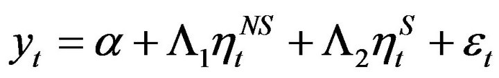 (6)
(6)
Proposition 1. Given model (6) and that ![]() is a
is a  non-stationary time series, the followings are equivalent:
1)  is cointegrated with rank r.
2)  is a stationary process. (existence of cointegration)
3) rank .
.
Therefore, testing the existence of cointegration can be achieved by testing whether the rank of  is smaller than Q. Note that the cointegration vector
  may not be unique, if there exist r such linearly independent
 , then
  is said to be cointegrated with cointegration rank r. It is worth mentioning that with two nonstationary time series,
  is unique if it exists and can be easily derived based on
 . And we call the ratio between the two time series as cointegration ratio in the following studies.
3. Bayesian Computation and Posterior Analysis
We use Markov Chain Monte Carlo (MCMC) sampler for the Bayesian inference of unknown quantities in the model. The sampler is computationally efficient and mixes rapidly due to the conditionally multivariate normal matrix state-space representation of the model as shown by (2). In details:
Let  denote all model parameters in (1), so that
 (7)
(7)
Also, recall that  defined in (2), with
  being a
  vector of initial values for the
  dynamic latent factor. Posterior inference is based on a standard Gibbs sampler that iteratively simulate from posterior full conditional distributions
 .
.
Specifically1) To sample from .
.
To obtain samples of latent factors  from the full conditional distribution, we applied a efficient sampler based on the Forward-Filtering-Backward-Sampling algorithm. Basically, forward filtering follows (2) and is performed in terms of
 . For backward sampling,
  is first sampled, giving samples of
 . Then
  are sequentially sampled backwardly based on the backward sampling distributions derived from model (1). The detailed filtering and sampling algorithm is shown in Appendix I.
2) To sample from .
.
Given latent factors  and the initial values
 , root structures
  are sampled following [6], from which samples of autoregression coefficients
  can be derived from the following equation:
where B is the backshift operator.
Given the half-cauchy priors for the innovation variances, posterior distributions of  do not have closed form, and thus are sampled using Adaptive-Rejection Sampler (ARS). Other model parameters generally have conjugate priors and have closed-form posteriors.
3) To sample from .
.
We take advantage of the reversibility of  process to sample initial values
 . So,
. So,
 (8)
(8)
Therefore, for the initial values
 of the
  latent factor,
are sequentially sampled backwardly from  to
to .
.
4. Simulation Examples
4.1. Study 1: Simulation from Factor Model
We first look at the case of detecting cointegration between two time series, where the time series  are generated from two latent dynamic latent factors
  , where
  follows random walk and
  follows a stationary
  process, as shown in (9).
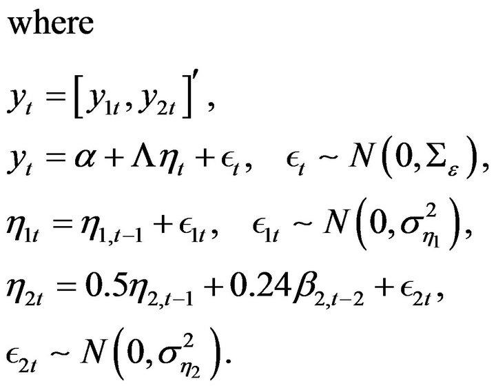 (9)
(9)
In the simulation study, we generated the times series of , and used
 ,
,  ,
,
 and
and . Clearly, in this case, the two time series cointegrate, with the cointegration ratio between
  and
and  being 5, meaning that zt = y1t + 5y2t is a stationary time series. To test the model we proposed for cointegration analysis, we modeled the simulated time series using a two-factor dynamic factor model as shown in (1), specifying the maximum number of pairs of complex roots to be 2, and that of real roots to be 4 for both dynamic latent factors. Thus, the maximum autoregressive order for both latent factors are 8. For efficient MCMC sampling, priors are placed on parameters of the Parameter-eXpanded (PX) model as described by [7] and [8]. 30,000 posterior samples are drawn for model parameters, latent initial values and latent factors via MCMC after a 5000 iteration burn-in.
Posterior inference of the existence of cointegration in this case is to test whether the rank of the factor loading matrix of non-stationary factors is smaller than 2. Therefore, we first looked at the posterior samples of the characteristic roots of both  and
and  and the factor loading matrix. Two results can be obtained immediately from this. First of all, based on 30,000 posterior samples, the marginal probability of
  having unit roots is
  and the joint probability of at least one of the latent factors having unit roots is
 , which are consistent with the known facts that both
  and
and  are non-stationary. Secondly, the probability that the rank of the factor loading matrix of non-stationary factors is smaller than the number of non-stationary component time series is
 , indicating that the two time series are cointegrated at the
 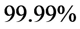 confidence level.
We also specifically focused on obtaining the conditional posterior distribution of the cointegration ratio  given the two cointegrate, which is an important quantity in cointegration analysis. This, in this case, can be derived from the posterior samples of roots and the factor loading matrix
 , as shown in Algorithm 1. A histogram of the posterior samples of
  is shown in Figure 1.
  has a posterior mean of 5.14, posterior mode of 5.03, and
 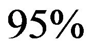 HPD interval of [4.47,5.79], which is consistent with the true values 5.
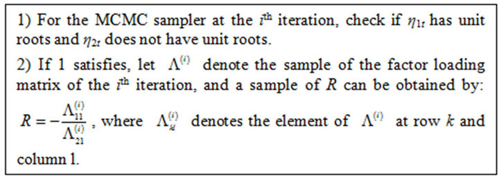
Algorithm 1. To derive posterior samples of the cointegration ratio (R) from .
.
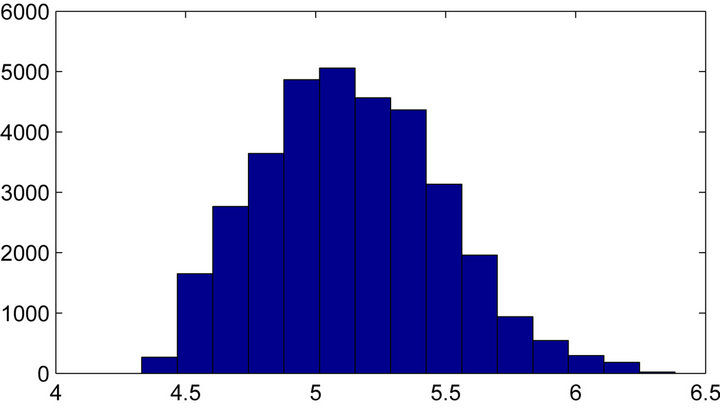
Figure 1. Histogram of posterior samples of cointegration ratio (R) shown, with true value being 5.
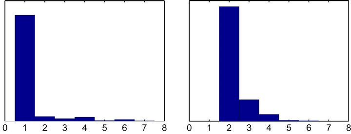
Furthermore, we looked at the inference of the latent factors structures. As shown in Table 1, the autoregression coefficients are all correctly inferred with posterior mean closed to and posterior C.I. covering the true values. Posterior distributions of autoregressive lag orders of both latent factors are also derived based on the non-zero posterior roots and the histograms are shown in Figure 2, which show good inference that the lag order of  spikes at 1 and that of
  peaks at 2.
Overall, the framework provides very good inference of the latent structures and unknown quantities. Cointegration relationship is also found correctly between the two non-stationary time series with good recovery of the cointegration ratio.
4.2. Study 2: Simulation from VECM Model
Out of model studies are shown here. We applied our model and algorithm to simulations generated from the Vector Error Correction Model (VECM). As stated earlier, the VECM representation has been commonly used for modeling and testing cointegration among I(1) nonstationary time series in both classical and Bayesian models.
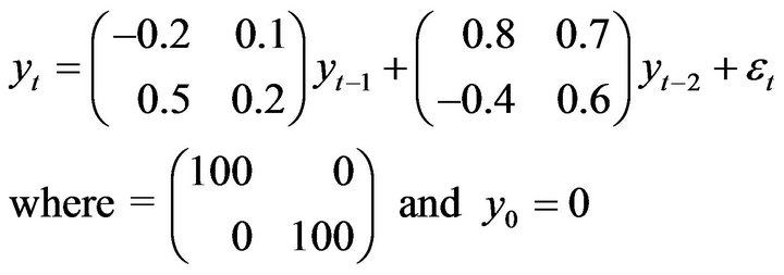
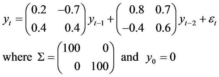
Taking advantage of the VECM model, an example of second-order nonstationary vector autoregressive model where cointegration exists is first considered here:
 (10)
(10)
This process gives the following VECM(2) represen-
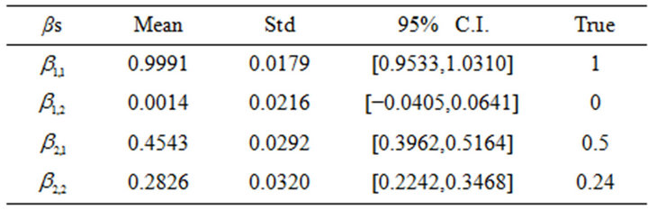
Table 1. Posterior summary of selected autoregression coefficients of latent factors, as compared to true values.
 (a) (b)
Figure 2. Histogram of posterior samples of autoregressive lag orders of latent factors η1t and η2t.
tation, indicating that the two time series are co-integrated, and the cointegration vector is 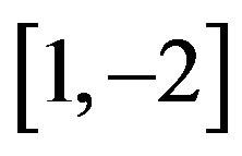 (with cointegration ratio being –2).
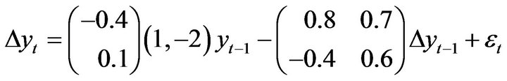 (11)
(11)
Our goal is to test whether our proposed framework can correctly detect the cointegration relationship between the time series and provide inference of other unknown quantities. We simulated the time series up to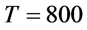 , with 8 time points of
  randomly missing. Two-factor model is fitted to the data, and set the maximum number of complex pairs and real roots to be 5 and 10 respectively, making the maximum autoregressive lag order being 20. Missing data are interpolated during MCMC. Similarly, PX-model are used for prior specification and posterior sampling, and 15,000 posterior samples of missing values, model parameters, root structures and latent factors are obtained via MCMC after a 5000 burn-in. First of all, the posterior marginal probability of having unit roots for the two latent factors are
 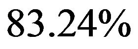 and
and , and the posterior joint probability of at least one of them have unit roots is
 , indicating that we cannot reject that both of the time series are nonstationary. Secondly, the existence of cointegration is tested. The posterior probability that the rank of the factor loading matrix of non-stationary factors is smaller than the number of unit-root processes is
 , indicating that cointegration exists at the
  confidence level.
Given that the test shows that the two time series cointegrate, we specifically analyze the cointegration ratio  between the two time series. Posterior distribution of the cointegration ratio are derived from posterior samples and plotted in Figure 3, with posterior mean at −2.060 and
  C.I.
C.I.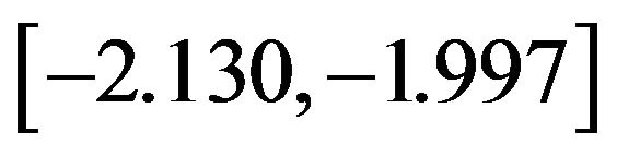 , This is very much consistent with the true value −2 (obtained from model (11)).
To confirm that the right posterior distribution of the cointegration ratio is found, we specifically focused on
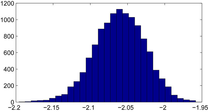
Figure 3. Histogram of posterior samples of cointegration ratio (R) shown.
the posterior mean , and let
 .
. ![]() is shown in Figure 4 to illustrate the mean-reverting property, the stationarity of which is further confirmed by Augmented Dickey-Fuller (ADF) test [9], which rejects the null hypothesis that
is shown in Figure 4 to illustrate the mean-reverting property, the stationarity of which is further confirmed by Augmented Dickey-Fuller (ADF) test [9], which rejects the null hypothesis that ![]() has unit roots with all p-values < 0.01 for lag orders up to 10.
has unit roots with all p-values < 0.01 for lag orders up to 10.
On the other hand, in a parallel study using the VECM model, two time series that are not co-integrated can be simulated from the following VAR model
 (12)
(12)
where the corresponding VECM representation is
 (13)
(13)
We also tested whether our model and algorithms can correctly detect the non-existence of the cointegration relationship between the time series, among inference of other unknown quantities. In this study, we simulated the two-dimensional time series up to , fit the data with two-factor model, and set the maximum number of complex pairs to be 10 and that of real roots to be 15 for both latent factors, suggesting that the maximum autoregressive lag order is 35. Based on 15,000 MCMC posterior samples of root structures and factor loading matrix after a 5000 burn-in, the posterior probability that the rank of the factor loading matrix of non-stationary factors is smaller than the number of unit-root processes is 4.44%, indicating that there is no existence of cointegration between the two time series at the 95% confidence level. Secondly, the posterior marginal probabilities of having unit roots for the two latent factors are 83.94% and 95.56%, and the posterior joint probability of at least one of them having unit roots is 99.36%, which means that we cannot reject that
  is nonstationary, and
  is non-stationary at 99% confident
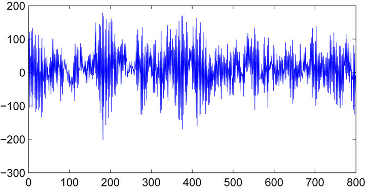
Figure 4. Plot of ![]() to illustrate mean-reverting and stationarity.
to illustrate mean-reverting and stationarity. , where R is the cointegration ratio, which is confirmed by formal ADF-test.
level.
Therefore, our simulation studies clearly show the efficacy of the model proposed to both capture the true (non)stationary strutures of the multivariate time series and identify the cointegration relationship correctly.
5. Real Data Analysis
5.1. GDX-GLD Pair vs PEP-KO Pair
Gold ETF GLD versus gold-miner ETF GDX have been reported as good candidates for real-world cointegrated pairs [10], because GLD reflects the spot price of gold, and GDX is a basket of gold-mining stocks. The cointegration relationship has been tested in empirical studies via frequentist cointegration test (e.g. Covariate-Augmented Dickey-Fuller (CADF) test), using the coefficient of the ordinary least squares regression as the cointegration ratio [11]. However, as mentioned earlier, most classical cointegration tests suffer from many problems, including multiple testing issues, how to choose lag order and whether deterministic terms (e.g. the intercept) should be included.
We applied our Bayesian cointegration analysis via dynamic factor models to the GDX and GLD daily closed price from Jun. 1, 2006 to Aug. 19, 2008 (T = 560). The original data (shown in Figure 5) is logtransformed, normalized and fitted with a two-factor dynamic factor model as (1), with priors placed on the corresponding PX-model. 15,000 posterior samples are obtained for each unknown quantity via MCMC and analyzed, after a 5000 burn-in.
Posterior samples show that the probability that the rank of the factor loading matrix of nonstationary factors is smaller than the number of unit-root process is 99.99%, indicating that based on this dataset the GDX and GLD
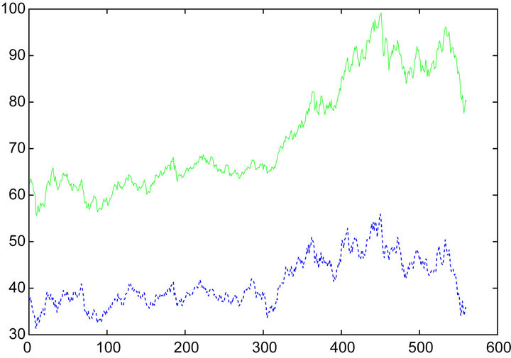
Figure 5. Original daily closed prices of GDX ETF (shown with the dotted line) and GLD ETF (shown with the solid line) from Jun. 1, 2006 to Aug. 19, 2008 are plotted. The original data is log-transformed and “normalized” before modeling.
cointegrate at the 99% confidence level. The marginal probability of the first latent factor having unit roots is 98.69%, and the joint probability of at least one factor having unit roots is 98.70%, showing that both time series are unit-root processes. Given that GDX and GLD cointegrate, the posterior samples of cointegration ratio  is calculated (
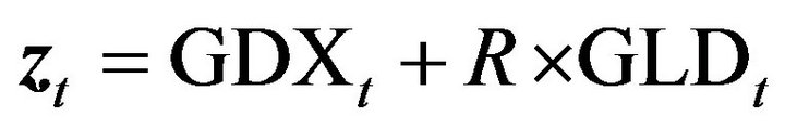 is stationary). R has the posterior mean of −0.8909 and 95% C.I. [−0.9290,−0.8524]. The histogram of R is shown in Figure 6.
To confirm that the right posterior distribution of R is found, we take the posterior mean , let
, let , and
, and ![]() is plotted in Figure 7 to illustrate the stationarity and mean-reversion. The stationarity of
is plotted in Figure 7 to illustrate the stationarity and mean-reversion. The stationarity of ![]() is further confirmed by testing the null hypothesis
is further confirmed by testing the null hypothesis  that the process
 ![]() has unit roots, using the Augmented Dickey-Fuller (ADF) test [9], and the p-values are shown in Table 2.
has unit roots, using the Augmented Dickey-Fuller (ADF) test [9], and the p-values are shown in Table 2.
Another candidate cointegrated pair could the stock price of PepsiCo Inc. (PEP) and Coca-Cola Co. (KO), because they operate in the same market and thus may be exposed to similar macro-economic and industry conditions. [11] specifically looked at this pair and showed
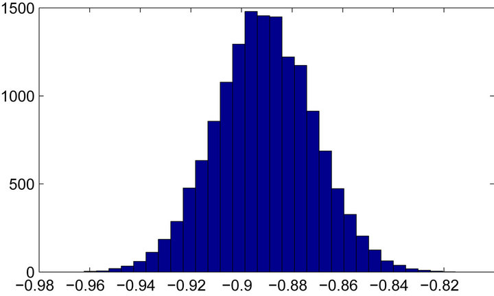
Figure 6. Histogram of posterior samples of cointegration ratio (R) between log-transformed GDX and GLD daily close price.
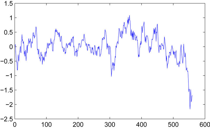
Figure 7. Plot of zt to illustrate stationarity. zt = GDX + R × GLD, where GDX and GLD are normalized log-transformed data, and R is the cointegration ratio.
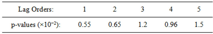
Table 2. p-Values of the ADF test for H0 with respect to different lag orders. H0:zt has unit roots.
that they are indeed correlated , but are not cointegrated, using the classical Augmented DickeyFuller (ADF) test. We also looked at the daily closed price of PEP and KO from Dec. 3, 1998 to Jan. 11, 2002
 . The log transformed data are fitted with the two-factor model, setting C = 5 and R = 10 (maximum autoregressive lag order of latent factors is thus 20). 15,000 posterior samples are obtained after a 5000 burnin, which shows that the probability that PEP and KO cointegrate is 1.6% and thus reject the existence of cointegration based on this dataset, which is also consistent to the finding of [11].
6. Conclusion
In this study, we showed the Bayesian factorized cointegration analysis for detecting cointegration among nonstationary time series. A strong message of this study is that, while testing cointegration of the original multivariate non-stationary time series via classical tests may have limitations both conceptually and computationally, studying the properties of independent latent factors in a Bayesian dynamic factor model framework serves as a powerful tool. As the majority of studies in the literature have used the traditional linear cointegrated error correction model, the models and methods we have described show accurate inference and efficient computation, and thus is a promising area for future research. One extension worth noting is to consider the more general case where the number of dynamic latent factors are unknown, in which the fundamental modeling and testing approaches discussed in this study are also applicable while some model selection criteria or penalization need to be further imposed to also incorporate the uncertainly of number of factors.
REFERENCES
- C. W. J. Granger and P. Newbold, “Spurious Regressions in Econometrics,” Journal of Econometrics, Vol. 2, No. 2, 1974, pp. 111-120.
- R. F. Engle and C. W. J. Granger, “Co-Integration and Error Correction: Representation, Estimation, and Testing,” Econometrica, Vol. 55, No. 2, 1987, pp. 251-276.
- S. Johansen, “Estimation and Hypothesis Testing of Cointegration Vectors in Gaussian Vector Autoregressive Models,” Econometrica, Vol. 59, No. 6, 1991, pp. 1551- 1580.
- M. West, “Time Series Decomposition,” Biometrika, Vol. 84, No. 2, 1997, pp. 489-494.
- A. Gelman, “Prior Distributions for Variance Parameters in Hierarchical Models,” Bayesian Analysis, Vol. 24, No. 1, 2006, pp. 1-19.
- G. Huerta and M. West. “Priors and Component Structures in Autoregressive Time Series Models,” Journal of the Royal Statistical Society Series B, Vol. 61, No. 4, 1999, pp. 881-899.
- J. Ghosh and D. B. Dunson, “Default Prior Distributions and Efficient Posterior Computation in Bayesian Factor Analysis,” Journal of Computational and Graphical Statistics, Vol. 18, No. 2, 2009, pp. 306-320.
- K. Cui and D. B. Dunson, “Generalized Dynamic Factor Models for Mixed-Measurement Time Series,” Journal of Computational and Graphical Statistics, 2012.
- D. A. Dickey and W. A. Fuller, “Distribution of the Estimators for Autoregressive Time Series with a Unit Root,” Journal of the American Statistical Association, Vol. 74, No. 366, 1979, pp. 427-431.
- K. Triantafyllopoulos and G. Montana, “Dynamic Modeling of Mean-Reverting Spreads for Statistical Arbitrage,” Computational Management Science, Vol. 8, No. 1-2, 2011, pp. 23-49.
- E. P. Chan, “Quantitative Trading,” John Wiley and Sons, Hoboken, 2008.
NOTES
1The roots are also the eigenvalues of A defined in (2).