Open Journal of Statistics
Vol.1 No.2(2011), Article ID:6182,12 pages DOI:10.4236/ojs.2011.12011
Distributions of Ratios: From Random Variables to Random Matrices*
Department of Mathematics and Statistics, Universite de Moncton, Canada
E-mail: #phamgit@umoncton.ca
Received March 25, 2011; revised April 17, 2011; accepted April 25, 2011
Keywords: Matrix Variate, Beta Distribution, Generalized-F Distribution, Ratios, Meijer G-Function, Wishart Distribution, Ratio
Abstract
The ratio R of two random quantities is frequently encountered in probability and statistics. But while for unidimensional statistical variables the distribution of R can be computed relatively easily, for symmetric positive definite random matrices, this ratio can take various forms and its distribution, and even its definition, can offer many challenges. However, for the distribution of its determinant, Meijer G-function often provides an effective analytic and computational tool, applicable at any division level, because of its reproductive property.
1. Introduction
In statistical analysis several important concepts and methods rely on two types of ratios of two independent, or dependent, random quantities. In univariate statistics, for example, the F-test, well-utilized in Regression and Analysis of variance, relies on the ratio of two independent chi-square variables, which are special cases of the gamma distribution. In multivariate analysis, similar problems use the ratio of two random matrices, and also the ratio of their determinants, so that some inference using a statistic based on the latter ratio, can be carried out. Latent roots of these ratios, considered either individually, or collectively, are also used for this purpose.
But, although most problems related to the above ratios are usually well understood in univariate statistics, with the expressions of their densities often available in closed forms, there are still considerable gaps in multivariate statistics. Here, few of the concerned distributions are known, less computed, tabulated, or available on a computer software. Results abound in terms of approximations or asymptotic estimations, but, as pointed out by Pillai ([1] and [2]), more than thirty years ago, asymptotic methods do not effectively contribute to the practical use of the related methods. Computation for hypergeometric functions of matrix arguments, or for zonal polynomials, are only in a state of development [3], and, at the present time , we still know little about their numerical values, to be able to effectively compute the power of some tests.
The use of special functions, especially Meijer G-functions and Fox H-functions [4] has helped a great deal in the study of the densities of the determinants of products and ratios of random variables, a domain not fully explored yet, computationally. A large number of common densities can be expressed as G-functions and since products and ratios of G-functions distributions are again G-functions distributions, this process can be repeatedly applied. Several computer applicable forms of these functions have been presented by Springer [5]. But it is the recent availability of computer routines to deal with them, in some commercial softwares like Maple or Mathematica, that made their use quite convenient and effective [6]. We should also mention here the increasing role that the G-function is taking in the above two softwares, in the numerical computation of integrals [7].
In Section 2 we recall the case of the gamma distribution and various results related to the ratio of two gammas in univariate statistics. In Section 3, going into matrix variate distributions, we consider first the classical case where both A and B are Wishart matrices, leading to the two types of matrix variate beta distributions for their ratios. The two associated determinant distributions are the two Wilks’s lambdas, with density expressed in terms of G-functions. It is of interest to note that the variety of special mathematical functions used in the previous section can all be expressed as G-functions, making the latter the only tool really required.
In Section 4, extensions of the results are made in several directions, to several Wishart matrices and to the matrix variate Gamma distribution. Several ratios have their determinant distribution established here, for example the ratio of a matrix variate beta distribution to a Wishart matrix, generalizing the ratio of a beta to a chi square. Two numerical examples are given and in Section 5 an example and an application are presented. Finally, although ratios are treated here, products, which are usually simpler to deal with, are also sometines studied.
2. Ratio of Two Univariate Random Variables
We recall here some results related to the ratios of two independent r.v.’s so that the reader can have a comparative view with those related to random matrices in the next section.
First, for , independent of
 ,
,  has density established numerically by Springer ([5], p. 148), using Mellin transform. Pham-Gia, Turkkan and Marchand ([8]) established a closed form expression for the more general case of the bivariate normal
 , using Kummer hypergeometric function
 . Springer ([5], p.156) obtained another expression but only for the case
 .
.
The gamma distribution,  , with density
 has as special case
  called the the Chi-square with n degrees of freedom
 , with density :
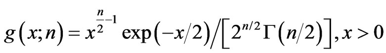 .
.
With independent Chi-square variables  and
and  , we can form the two ratios
  and
and  which have, respectively, the standard beta distribution on [0,1] (or beta of the first kind
 , with density defined on
  by:
by:
 ,
, .
.
and standard betaprime distribution ( beta of the second kind ) defined on
  by
by
 .
.
The Fisher-Snedecor variable  is just a multiple of the univariate beta prime
 .
.
For independent , we can form the same ratios
  and
and .
.  has the Generalized-F distribution,
  , with density :
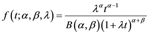 where
where  and we have
 .
.
Naturally, when ,
,  and
and .
.
Starting now from the standard beta distribution defined on (0,1), Pham-Gia and Turkkan [9] give the expression of the density of R, and also of , using Gauss hypergeometric function
 . For the general beta defined on a finite interval (a,b), Pham-Gia and Turkkan [10] gives the density of R, using Appell’s function
 , a generalization of
 . In [11], several cases are considered for the ratio X/Y, with
 . In particular, the Hermite and Tricomi functions,
  and
and , are used. The Generalized-F variable being the ratio of two independent gamma variables, its ratio to an independent Gamma is also given there, using
 . Finally, the ratio of two independent Generalized-F variables is given in [11], using Appell function
  again. All these operations will be generalized to random matrices in the following section.
3. Distribution of the Ratio of Two Matrix Variates
3.1. Three Types of Distributions
Under their full generality, rectangular (p × q) random matrices can be considered, but to avoid several difficulties in matrix operations and definitions, we consider only symmetric positive definite matrices. Also, here, we will be concerned only with the non-singular matrix, with its null or central distribution and the exact, non-asymptotic expression of the latter.
For a random (p × q) symmetric matrix, , there are three associated distributions. We essentially distinguish between:
1) the distribution of its elements (i.e. its  independent elements
  in the case of a symmetric matrix), called here its elements distribution (with matrix input), for convenience. This is a mathematical expression relating the components of the matrix, but usually, it is too complex to be expressed as an equation (or several equations) on the elements
  themselves and hence, most often, it is expressed as an equation on its determinant.
2) the univariate distribution of its determinant (denoted here by  instead of
 ) (with positive real input), called determinant distribution, and 3) the distribution of its latent roots (with p-vector input), called latent roots distribution.
These three distributions evidently become a single one for a positive univariate variable, then called its density. The literature is mostly concerned with the first distribution [12] than with the other two. The focal point of this article is in the determinant distribution.
3.2. General Approach
When dealing with a random matrix, the distribution of the elements within that random matrix constitutes the first step in its study, together with the computation of its moments, characteristic function and other properties.
Let X and Y be two symmetric, positive definite independent (p × q) random matrices with densities (or elements distributions)  and
and . As in univariate statistics, we first define two types of ratios, type I of the form
 , and type II, of the form:
 . However, for matrices, there are several ratios of type II that can be formed:
 ,
,  and
and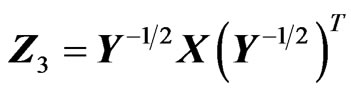 , where
  is the symmetric square root of Y, i.e.
 , beside the two formed with the Cholesky decomposition of Y,
 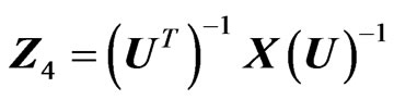 and
and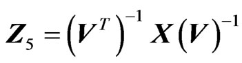 , where U is upper triangular, with
 , and V, lower triangular, with
 .
.
1) For elements distribution, we only consider , which is positive and symmetric, but there are applications of
  and
and  in the statistical literature. We can determine the matrix variate distribution of
  from those of X and Y. In general, for two matrix variates A and B, with joint density
  the density of
  is obtained by a change of variables:
 , with dA associated with all elements of A. When A and B are independent, we have
 .
.
Gupta and Kabe [13], for example, compute the density of G from the joint density , using the approach adopted by Phillips [14].
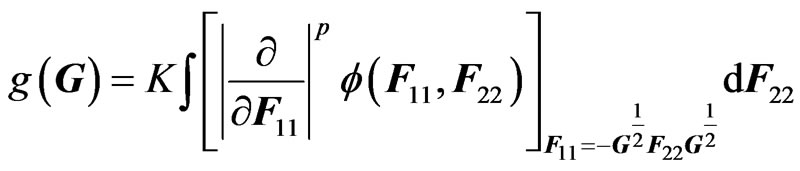 where in the block division of A,
 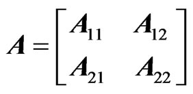 , we have:
  while
while  is the joint characteristic function of
  et
et .
.
For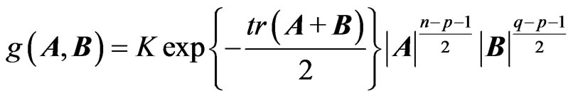 they obtained
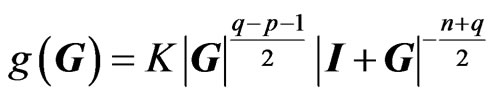 , i.e.
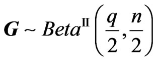 .
.
Similarly, for Type I ratio, we can also have 5 types of ratios, and we will consider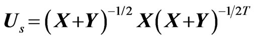 , the symmetric form of the ratio
  for elements distribution.
2) In general, the density of the determinant of a random matrix , can be obtained from its elements distribution
  of the previous section, in some simple cases, by using following relation for differentials:
  ([15], p. 150). In practice, frequently, we have to manipulate
  directly, often using an orthogonal transformation, to arrive at a product of independent diagonal and off-diagonal elements.
The determinants of the above different ratios , have univariate distributions that are identical, however, and they are of much interest since they will determine the null distribution useful in some statistical inference procedures.
3) Latent roots distributions for ratios, and the distributions of some associated statistics, remain very complicated, and in this article, we just mention some of their basic properties. For the density of the latent roots , we have, using the elements density
 :
:
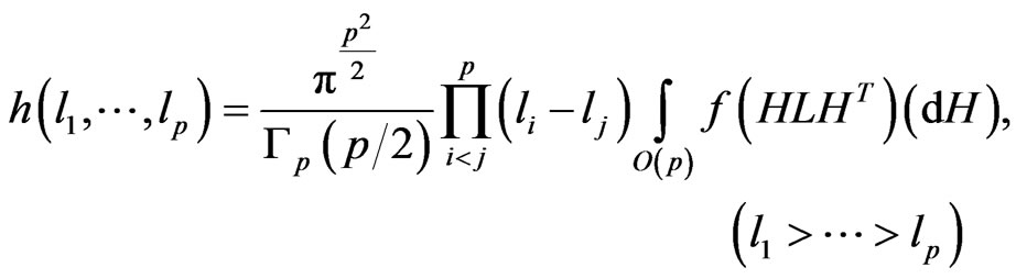
where  is the orthogonal group,
  is an orthogonal
  matrix,
  is the Haar invariant measure on
 , and
, and  ([16], p. 105).
3.3. Two Kinds of Beta, of Wilks’s Statistic, and of Latent Roots Distributions
We examine here the elements, determinant and latent roots distributions of a random matrix called the beta matrix variate, the homologous of the standard univariate beta.
First, the Wishart distribution, the matrix generalization of the chi-square distribution, played a critical part in the development of multivariate statistics. , is called a Wishart Matrix with parameters n and C if its density is:
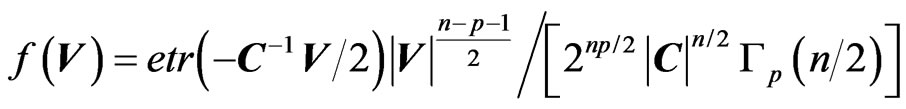 (1)
(1)
 . It is a particular case of the Gamma matrix variate
 , with matrix density:
 (2)
(2)
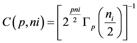
with  and
and 
Hence, If , then
 .
.
THEOREM 1: Let  et
et , with A and B independent
  positive definite symmetric matrices, and
  and
and  integers, with
 . Then, for the three above-mentioned distributions, we have:
3.3.1. Elements Distribution
1) The ratio  has the matrix beta distribution
 , with density given by (3).
2) Similarly, the ratio  has a
has a  distribution if
  and
and  is symmetric. Its density is given by (4).
3.3.2. Determinant Distribution
1) For , its determinant
  has Wilks’s distribution of the first type, denoted by
 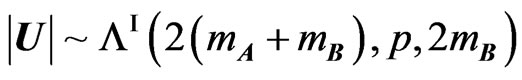 (to follow the notation in Kshirsagar [17], expressed as a product of independent
 , and its density, is given by (5).
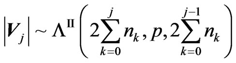
2) For , its determinant
  has Wilks’s distribution of the second type, denoted by
 , expressed as a product of p independent univariate beta primes
 , and its density is given by (6).
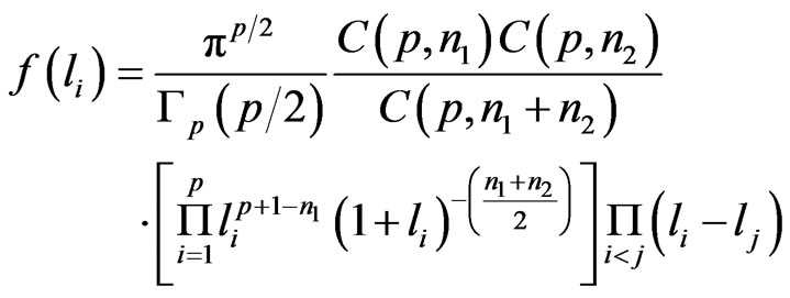
3.3.3. Latent Roots Distribution
1) The latent roots of U: The null-density of the latent roots  of
of 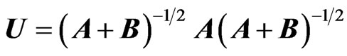
 or
or 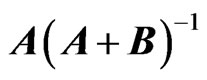 is:
is:
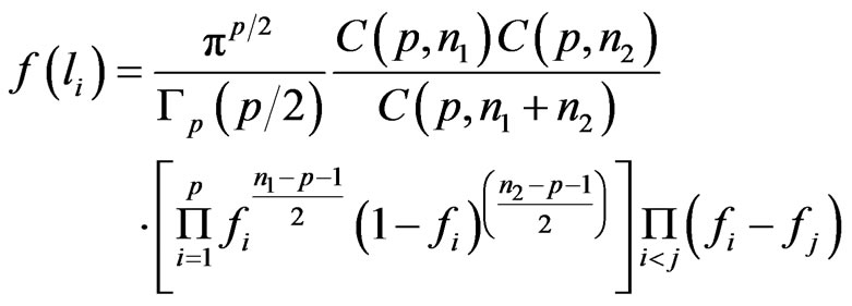
defined in the sector , with
 where
where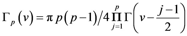 ,(If
,(If 
but , we can make the changes
 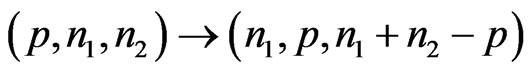 to obtain the right expression).
2) The latent roots of V: For 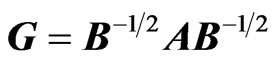 or
or , the roots
  have density:
We have also: .
.
PROOF: The proofs of part 1) and part 3) are found in most textbooks in multivariate analysis. For part 2, see [6]. QED.
The following explicative notes provide more details on the above results.
3.4. Explicative Notes
1) On Elements Distributions: The positive definite symmetric random matrix U has a beta distribution of the first kind,  if its density is of the form:
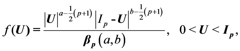 (3)
(3)
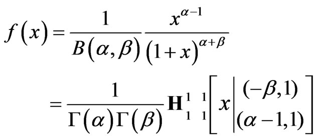
It has a beta of the second kind distribution, denoted by  if its density is of the form:
![]()
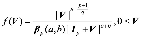 (4)
(4)
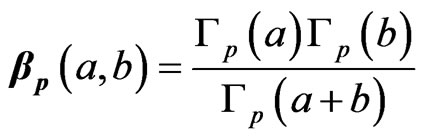
where , are positive real numbers, and
  is the beta function in
 , i.e.
 , with
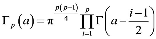 .
.
The transformations from  to
to  and vice-versa are simple ones, Also, similarly to the univariate case, where the beta prime is also called the gamma-gamma distribution, frequently encountered in Bayesian Statistics [11],
  can also be obtained as the continuous mixture of two Wishart densities, in the sense of
  with
with . Also, for U and V above,
  and
and .
.
2) For the general case where , V is not necessarily
 , as pointed out by Olkin and Rubin [18]. Several other reasons, such as its dependency on
  and on (A + B), makes V difficult to use, and Perlman [19] suggested using
  which does not have these weaknesses. We will use this definition as the matrix ratio type II of A and B when considering its elements distribution.
2) On Determinant Distributions: a) For  its determinant
  has Wilks’s distribution of the first type, denoted by
  (to follow the notation in [17]), expressed as a product of p univariate betas of the first kind, and this expression has been treated fully in [6]. This result is obtained via a transformation and by considering the elements on the diagonal.
PROPOSITION 1: For integers  and
and , with
 a) The density of the ratio
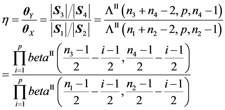
 , is: (see (5)).
where .
.
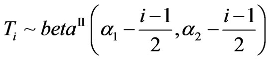
b) For , the latent roots of
 ,
,  , and
, and  are the same, and so are the three determinants, and
  can be expressed as a product of p independent univariate beta primes, which, in turn, can be expressed as Meijer’s G-functions, i.e.
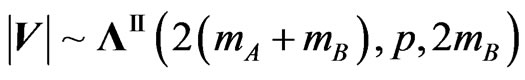 , or the Wilks’s distribution of the second type . Hence, for the above ratio V
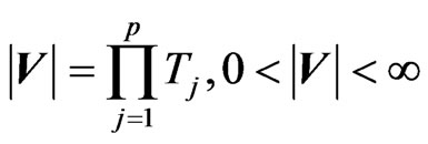 , with
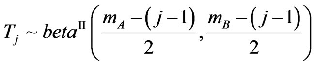 where
where  if it has as univariate density
 (6)
(6)
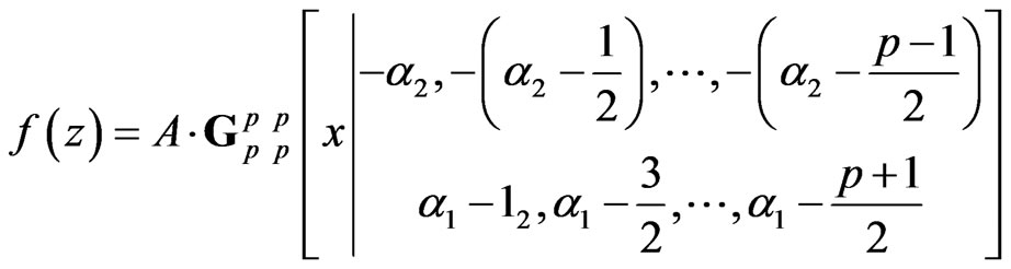
PROPOSITION 2: Wilks’s statistic of the second kind,  , has as density (see (7)).
with .
.
In the general case  can have non-integral values and we can also have the case
 .
.
PROOF: See (6).
REMARK: The cdf of Y is expressible in closed form, using the hypergeometric function  of matrix argument. ([12], p. 166) and the moments are
 for
for
3) On Latent Roots distributions:
The distribution of the latent roots  of
of  was made almost at the same time by five distinguished statisticians, as we all know. It is sometimes referred to as the generalized beta, but the marginal distributions of some roots might not be univariate beta. Although they are difficult to handle, partially due to their domain of definition as a sector in
 , their associations with the Selberg integral, as presented in [20], has permitted to derive several important results. A similar expression applies for the latent roots of
 .
.
4. Extensions and Generalizations
From the basic results above, extensions can be made into several directions and various applications can be found. We will consider here elements and determinant distributions only. Let us recall that for univariate distributions there are several relations between the beta and the Dirichlet, and these relations can also be established for the matrix variate distribution.
 (5)
(5)
 (7)
(7)
4.1. Extensions
4.1.1. To Several Matrices
There is a wealth of relationships between the matrix variate Dirichlet distributions and its components [12], but because of space limitation, only a few can be presented here. The proof of the following results can be found in [18] and [19], where the question of independence between individual ratios and the sum of all matrices is discussed.
1) In Matrix-variate statistics, if  are (k + 1) independent (p × p) random Wishart matrices,
 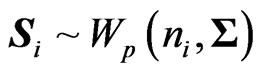 , then, the matrix variates
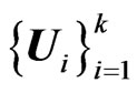 , defined “cumulatively” by:
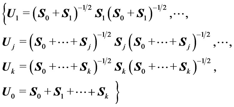
are mutually independent, with , having a matrix variate beta distrib.
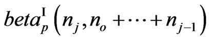 .
.
2) Similarly, as suggested by Perlman [19], defining,
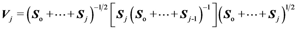
then  and are mutually independent. Concerning their determinants, we have:
THEOREM 2: Let  be (k + 1) indep (p × p) random Wishart matrices and
  and
and 
defined as above. Then the two products  and
and 
 , as well as any ratio
 and
and , have the densities of their determinants expressed in closed forms in terms of Meijer G-functions.
PROOF: We have ,
, 
 , and the result is immediate from Section 2 of Theorem 1 and the expression of the G-function for products and ratios of independent G-function distributions given in the Appendix. Exact expressions are not given here to save space but are available upon request.
QED.
Also, considering the sum , if we take:
 ,
,  and
and 
 , then
1) the matrix vector  has the matrix variate Dirichlet of type I distribution, i.e.
 , with density:
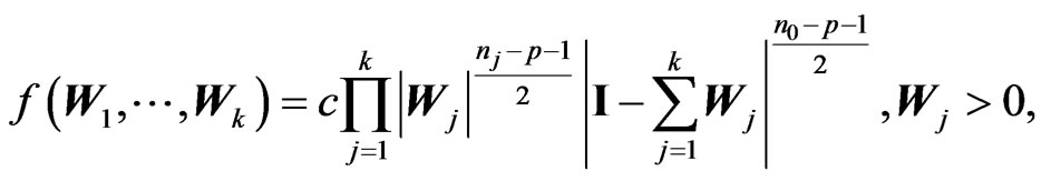
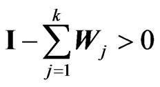 , where
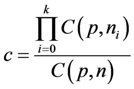 , with
  and
and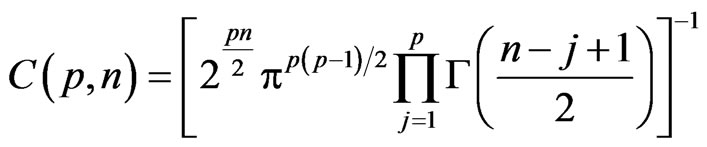 .
.
and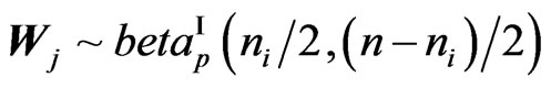 .
.
2) the matrix vector ( ) has the matrix variate Dirichlet of type II distribution, i.e.
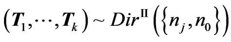 , with density:
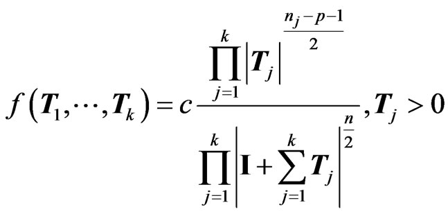
and .
.
THEOREM 3: Under the same hypothesis as Theorem 2 the densities of the determinants of  and of
 , can be obtained in closed form in terms of G-functions.
PROOF: We have  and
and ,
,  and the conclusion is immediate from Section 2 of Theorem 1.
QED.
4.1.2. To the Matrix Variate Gamma Distribution
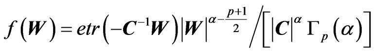
In the preceding sections we started with the Wishart distribution. However, it is a more general to consider the Gamma matrix variate distribution, .
.
Here, we know that , with independent
 . Hence, the density of
  is :
is :
 (8)
(8)
with .
.
Although for two independent Matrix Gammas,  and
and , their symmetric ratio of the second type,
 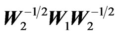 , suffers from the same definition difficulty as with the Wishart, the same recommendations made by Perlman [19] can be implemented to obtain the well-defined elements distribution of the Generalized F Matrix variate
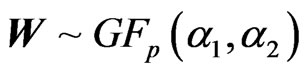 . The matrix variate
  -distribution, a scaled form of the
 , is encountered in multivariate regression, just like its univariate counterpart. But we have, for the ratio of the two determinants
 , with independent
 (9)
(9)
Hence, the distribution of , the determinant of
  has density:
 (10)
(10)
with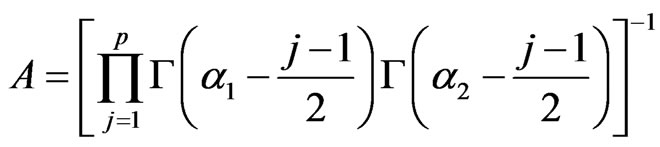 , which is of the same form as (4).
The determinants of the product and ratio of the two  variates, can now be computed, using the method given in the Appendix, extending the univariate case established for the generalized-F [11].
4.2. Further Matrix Ratios
There are various types of ratios encountered in the statistical literature, extending the univariate results of Pham-Gia and Turkkan [21] on divisions by the univariate gamma variable. We consider the following four matrix variates, which include all cases considered previously ( is a special case of
 ):
):
Let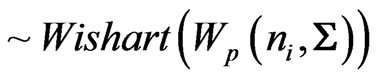
 , with integer n,
  Beta type I (
 ),
), Beta type II or GFp (a,b) (
 or
or ),
),  ,
,  Gamma
Gamma  (
( ).
).
The elements distributions of various products , and ratios
  and
and
 , for independent
 ,
,
 , can be carried out, but will usually lead to quite complex results. Some results when both
  and
and  are
are  -matrices are obtained by Bekker, Roux and Pham-Gia [22].
However, for their determinants, we have:
 ,
,
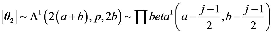 ,
, 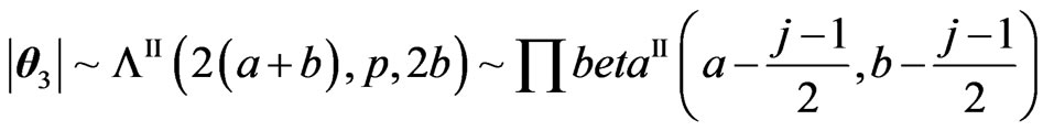 ,
,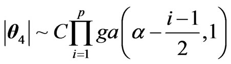 .
.
The expressions of the densities of , in terms of G-functions are given in previous sections, except for
  the density of which is given by (12) below.
  and
and  here are generalized Wilks’s variables, with a and b positive constants, instead of being integers.
THEOREM 4: For any of the above matrix variates 
a) The density of the determinant of any product  =
= , and ratio
  =
= ,
,  , in the above list, can be expressed in terms of Meijer G-functions.
b) Furthermore, subject to the independence of all the factors involved, any product and ratio of different , and of different
  and
and ,
,  , can also have their densities expressed in terms of G-functions.
PROOF: The proof is again based on the reproductive property of the Meijer G-functions when product and ratio operations are performed, with the complex expressions for these operations presented in [6], and reproduced in the Appendix. Computation details can be provided by the authors upon request.
QED.
REMARK: Mathai [23] considered several types of integral equations associated with Wilks’ work and provide solutions to these equations in a general theoretical context. The method presented here can be used to give a G-function or H-function form to these solutions, that can then be used for exact numerical computations.
5. Example and Application
We provide here an example using Theorem 4, with two graphs and also an engineering application.
5.1. Example
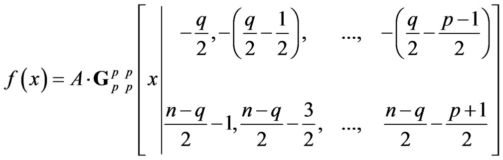
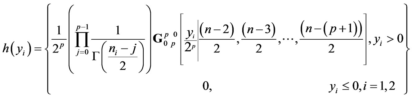
Let . The densities of Y =
  and R =
  can be obtained in closed form as follows:
 (11)
(11)
for  with
with ,
,  and
and ,
, .
.
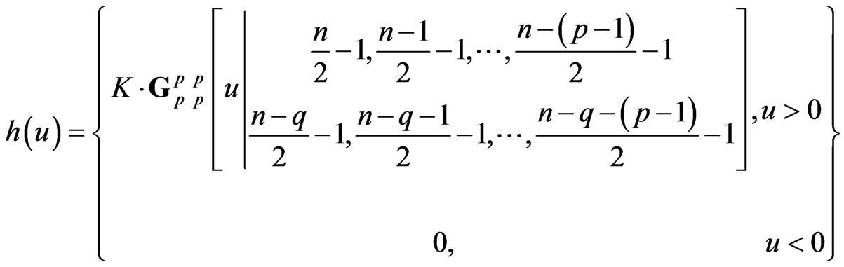
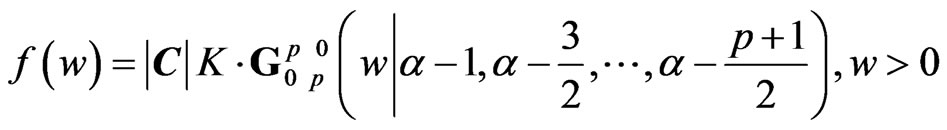
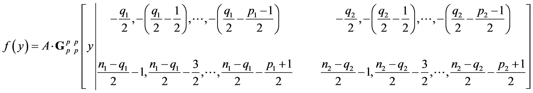
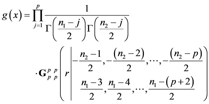
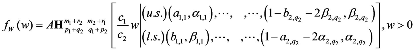
Similarly, the ratio R has density:
 (12)
(12)
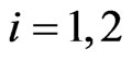
for .
.
PROOF: Using (7) above, we can derive (11) and (12) by applying the approach presented in the Appendix.
QED.
Figure 1 and Figure 2 give, respectively, these two densities, for  and
and  18, using the MAPLE software.
5.2. Application to Multivariate Process Control
1) Ratios of Variances: The generalized variance is treated in [24]. We consider  and a random sample
  of X. We define
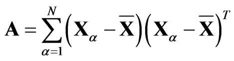 , the sample sum of squares and products matrix, and the sample covariance matrix
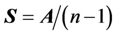 . We have:
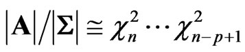 (13)
(13)
where the  variables, with j degrees of freedom,
  are independent.
This is also the distribution of .
.
Now let  and
and  be two independent sample covariance matrices of sizes
  and
and  respectively. From (1), we have
 .
.
a) The sample generalized variance  has density:
 (14)
(14)
2) Now, the two types of ratios V =  and U =
 , can be determined.
We have 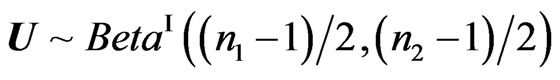 and
and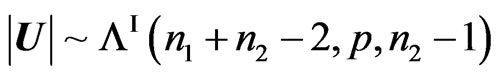 . V has a density which is not necessarily
 , but we have:
 .
.
2) Application: In an industrial environment we wish to monitor the variations of a normal process X , using the variations of the ratio of two random sample covariance matrices taken from that environment, against the fluctuations of its control environment Y
 , represented by a similar ratio.
For clarity, we will proceed in several steps:
a) Let , with
  and
and  being two random samples of sizes
  and
and  from
from  and, similarly,
  , with
  and
and  being two random samples of sizes
  and
and 
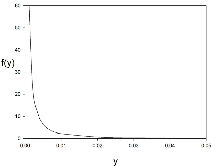
Figure 1. Density of , with
 .
.
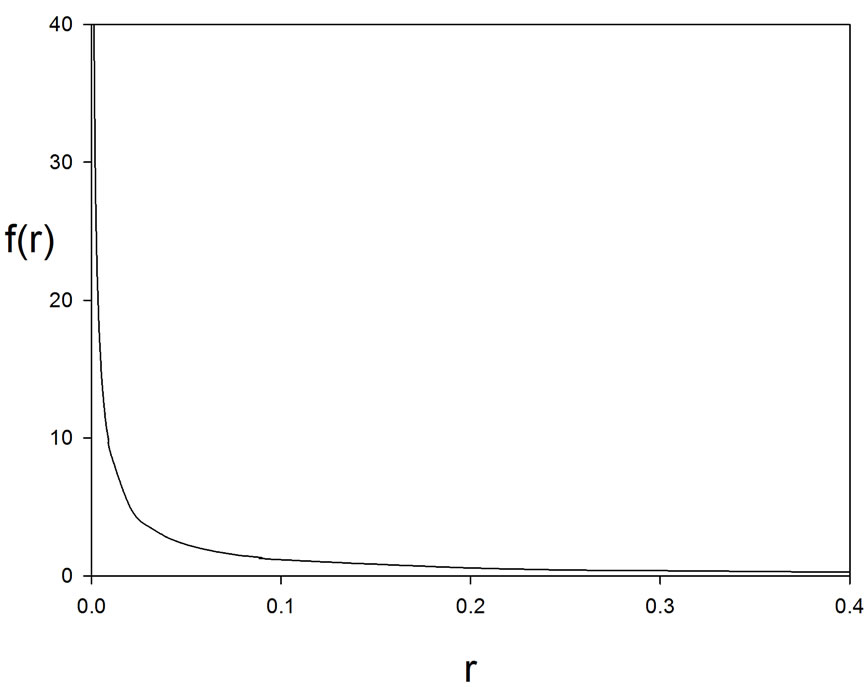
Figure 2. Density of .
.
from . Hence,
b) For the denominator, its density is given by (7):
and similarly for the numerator.
c) Applying the ratio rule in the Appendix for these two independent G-function distributions, we have the density of .
.
QED.
6. Conclusions
As shown in this article, for several types of random matrices, the moments of which can be expressed in terms of gamma functions, Meijer G-function provides a powerful tool to derive, and numerically compute, the densities of the determinants of products and ratios of these matrices. Multivariate hypothesis testing based on determinants can now be accurately carried out since the expressions of null distributions are, now, not based on asymptotic considerations.
7. References
[1] K. C. S. Pillai, “Distributions of Characteristic Roots in Multivariate Analysis, Part I: Null Distributions,” Communications in Statistics—Theory and Methods, Vol. 4, No. 2, 1976, pp. 157-184.
[2] K. C. S. Pillai, “Distributions of Characteristic Roots in Multivariate Analysis, Part II: Non-Null Distributions,” Communications in Statistics—Theory and Methods, Vol. 5, No. 21, 1977, pp. 1-62.
[3] P. Koev and A. Edelman, “The Effective Evaluation of the Hypergeometric Function of a Matrix Argument,” Mathematics of Computation, Vol. 75, 2006, pp. 833-846. doi:10.1090/S0025-5718-06-01824-2
[4] A. M. Mathai and R. K. Saxena, “Generalized Hypergeometric Functions with Applications in Statistics and Physical Sciences,” Lecture Notes in Mathematics, Vol. 348, Springer-Verlag, New York, 1973.
[5] M. Springer, “The Algebra of Random Variables,” Wiley, New York, 1984.
[6] T. Pham-Gia, “Exact Distribution of the Generalized Wilks’s Distribution and Applications,” Journal of Muotivariate Analysis, 2008, 1999, pp. 1698-1716.
[7] V. Adamchik, “The Evaluation of Integrals of Bessel Functions via G-Function Identities,”Journal of Computational and Applied Mathematics, Vol. 64, No. 3, 1995, pp. 283-290. doi:10.1016/0377-0427(95)00153-0
[8] T. Pham-Gia, T. N. Turkkan and E. Marchand, “Distribution of the Ratio of Normal Variables,” Communications in Statistics—Theory and Methods, Vol. 35, 2006, pp. 1569-1591.
[9] T. Pham-Gia and N. Turkkan, “Distributions of the Ratios of Independent Beta Variables and Applications,” Communications in Statistics—Theory and Methods, Vol. 29, No. 12, 2000, pp. 2693-2715. doi:10.1080/03610920008832632
[10] T. Pham-Gia and N. Turkkan, “The Product and Quotient of General Beta Distributions,” Statistical Papers, Vol. 43, No. 4, 2002, pp. 537-550. doi:10.1007/s00362-002-0122-y
[11] T. Pham-Gia and N. Turkkan, “Operations on the Generalized F-Variables, and Applications,” Statistics, Vol. 36, No. 3, 2002, pp. 195-209. doi:10.1080/02331880212855
[12] A. K. Gupta and D. K. Nagar, “Matrix Variate Distributions,” Chapman and Hall/CRC, Boca Raton, 2000.
[13] A. K. Gupta and D. G. Kabe, “The Distribution of Symmetric Matrix Quotients,” Journal of Multivariate Analysis, Vol. 87, No. 2, 2003, pp. 413-417. doi:10.1016/S0047-259X(03)00046-0
[14] P. C. B. Phillips, “The Distribution of Matrix Quotients,” Journal of Multivariate Analysis, Vol. 16, No. 1, 1985, pp. 157-161. doi:10.1016/0047-259X(85)90056-9
[15] A. M. Mathai, “Jacobians of Matrix Transformations and Functions of Matrix Argument,” World Scientific, Singapore, 1997.
[16] R. J. Muirhead, “Aspects of Multivariate Statistical Theory,” Wiley, New York, 1982. doi:10.1002/9780470316559
[17] A. Kshirsagar, “Multivariate Analysis,” Marcel Dekker, New York, 1972.
[18] I. Olkin and H. Rubin, “Multivariate Beta Distributions and Independence Properties of the Wishart Distribution,” Annals Mathematical Statistics, Vol. 35, No.1, 1964, pp. 261-269. doi:10.1214/aoms/1177703748
[19] M. D. Perlman, “A Note on the Matrix-Variate F Distribution,” Sankhya, Series A, Vol. 39, 1977, pp. 290-298.
[20] T. Pham-Gia, “The Multivaraite Selberg Beta Distribution and Applications,” Statistics, Vol. 43, No. 1, 2009, pp. 65-79. doi:10.1080/02331880802185372
[21] T. Pham-Gia and N. Turkkan, “Distributions of Ratios of Random Variables from the Power-Quadratic Exponential family and Applications,” Statistics, Vol. 39, No. 4, 2005, pp. 355-372.
[22] A. Bekker, J. J. J. Roux and T. Pham-Gia, “Operations on the Matrix Variate Beta Type I Variables and Applications,” Unpublished Manuscript, University of Pretoria, Pretoria, 2005.
[23] A. M. Mathai, “Extensions of Wilks’ Integral Equations and Distributions of Test Statistics,” Annals of the Institute of Statistical Mathematics, Vol. 36, No. 2, 1984, pp. 271-288.
[24] T. Pham-Gia and N. Turkkan, “Exact Expression of the Sample Generalized Variance and Applications,” Statistical Papers, Vol. 51, No. 4, 2010, pp. 931-945.
Appendix
The H-function  is defined as follows:
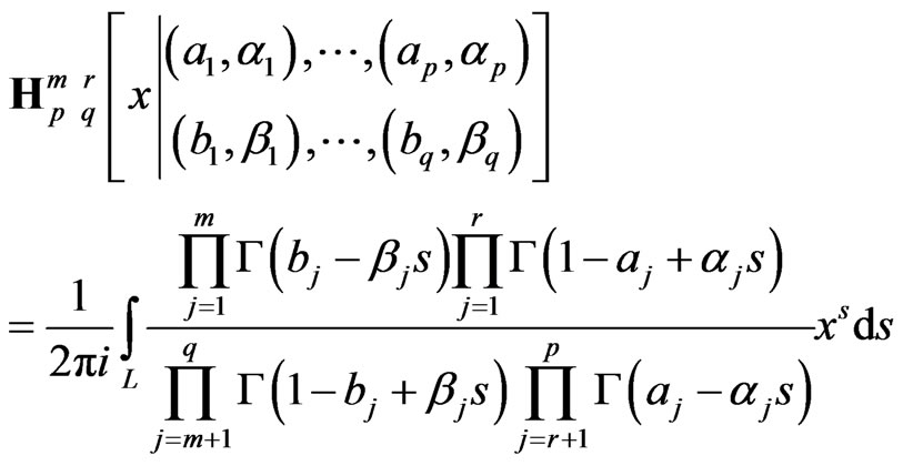 i.e. it is the integral along the complex contour L of a ratio of products of gamma functions. H-function has a relationship with the generalized hypergeometric function:
 . An equivalent form is obtained by replacing s by (-s), which shows that the integrant is, in fact, a Mellin-transform. Numerically, H-functions can be computed by using the residue theorem in complex analysis, together with Jordan’s lemma, but because of the complexity of this operation, it is only quite recently that it is available on softwares, although, in the past, several authors have suggested their own versions in their published works.
In this Appendix, the densities of the product and ratio of two independent random variables, whose densities are expressed in H-functions, is obtained. For G-functions, we have , and since these values are not affected by the operations the following results remain valid.
1) Product: Let , be s independent H-function random variables , each with pdf :
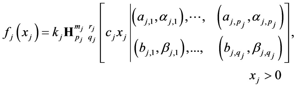 (6)
(6)
The product of these variables, 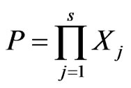 , is also a H-Function Random variable, with density
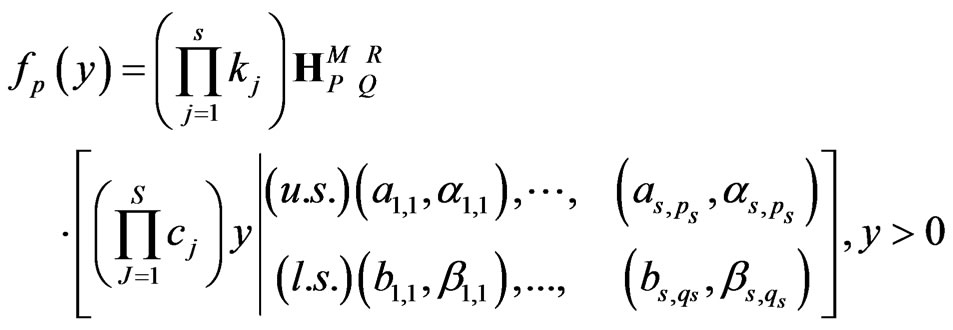 (7)
(7)
where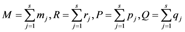 , and the two parameter sequences, (u.s.) and (l.s.), are as follows:
a) The upper sequence of parameters (u.s.), of total length P, consists of s consecutive subsequences of the type , followed by s consecutive subsequences of the type
 , i.e. we have:
 (8)
(8)
b) Similarly, the lower parameter sequence (l.s.), of total length Q, consists of s consecutive subsequences of the type , followed by s consecutive subsequences of the type:
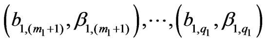 , i.e. we have:
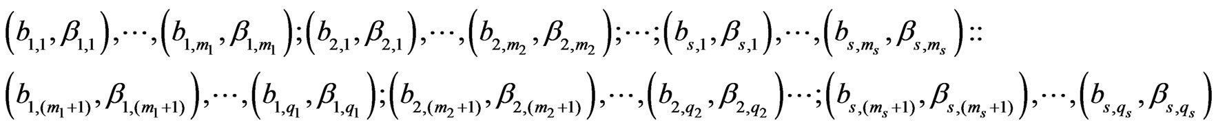 (9)
(9)
2) Ratio: For the ratio , its density is:
 (10)
(10)
where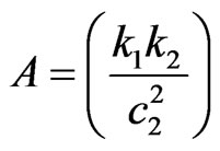 .
.
a) The upper sequence of parameters (u.s.), of total length , consists of the four consecutive subsequences:
 of length
 of length
  (11)
(11)
 of length
 , and
, and
 of length
 .
.
b) The lower sequence (l.s.), of total length , also has 4 subsequences of respective lengths
  and
and :
:

 , (12)
 , and
, and
 .
.
PROOF: The proofs of the above results, based on the Mellin transform of a function  defined on
 , and its inverse Mellin transform , as defined previously, are quite involved, but can be found in Springer (1984, p. 214).
QED.
NOTES
*Research partially supported by NSERC grant A9249 (Canada).