American Journal of Computational Mathematics
Vol.2 No.1(2012), Article ID:17967,5 pages DOI:10.4236/ajcm.2012.21007
An Improved Kriging Interpolation Technique Based on SVM and Its Recovery Experiment in Oceanic Missing Data*
Institute of Meteorology, PLA University of Science and Technology, Nanjing, China
Email: hzsong123@126.com
Received December 24, 2011; revised January 25, 2012; accepted February 3, 2012
Keywords: Least Square Support Vector Machine; Kriging Interpolation; Variogram; SVM-Kriging
ABSTRACT
In Kriging interpolation, the types of variogram model are very finite, which make the variogram very difficult to describe the spatial distributional characteristics of true data. In order to overcome its shortage, an improved interpolation called Support Vector Machine-Kriging interpolation (SVM-Kriging) was proposed in this paper. The SVM-Kriging uses Least Square Support Vector Machine (LS-SVM) to fit the variogram, which needn’t select the basic variogram model and can directly get the optimal variogram of real interpolated field by using SVM to fit the variogram curve automatically. Based on GODAS data, by using the proposed SVM-Kriging and the general Kriging based on other traditional variogram models, the interpolation test was carried out and the interpolated results were analyzed contrastively. The test show that the variogram of SVM-Kriging can avoid the subjectivity of selecting the type of variogram models and the SVM-Kriging is better than the general Kriging based on other variogram model as a whole. Therefore, the SVM-Kriging is a good and adaptive interpolation method.
1. Introduction
Kriging is a method of interpolation which predicts unknown values from data observed at known locations, and it minimizes the error of predicted values which are estimated by spatial distribution of the predicted values. Kriging uses variogram to express the spatial variation. The key problem of Kriging is selection of variogram model, which determines the spatial interpolation accuracy. Variogram model includes linear model, exponenttial model, Gaussian model, spherical model and so on. In a general way, the reasonable variogram model is selected based on the cloud pictures of variogram distribution. However, this general method of variogram selection is subjective, and may not select the optimal variogram model.
In order to overcome the shortcoming of variogram model selection, an improved interpolation method called Support Vector Machine-Kriging interpolation (SVMKriging) was proposed. SVM-Kriging uses least square support vector machine (LS-SVM) to fit the variogram, which needn’t select the basic variogram model and can directly get the optimal variogram of real interpolated field by using SVM to fit the variogram curve automatically. The variogram of SVM-Kriging come from the real data, so it can avoid the subjectivity and arbitrariness of selecting the type of variogram models and improve the interpolated results. Based on GODAS data, the proposed SVM-Kriging was compared with other general variogram models in this paper.
2. General Kriging
2.1. Basic Idea
Let  be the value of the variable
  at a point
 . Given the n measurements
  at known locations
 , you want to obtain an estimate of
  at an unsampled location
 .
.
The Kriging estimator is given by weighed linear combinations of the available samples [1]:
 (1)
(1)
Considering the unbiasedness condition yields:
 (2)
(2)
Under this condition, the variance of estimate error of expression can be simplified as follows:
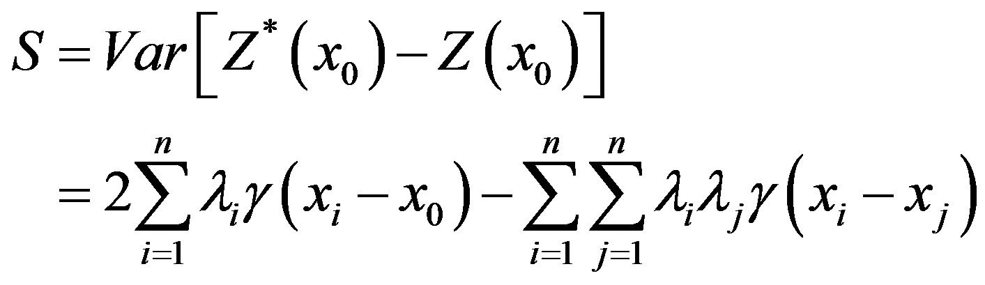 (3)
(3)
where  is variogram. Under the restricted condition (2), in order to make the estimate variance minimum, by introducing Lagrange multiplier, the Kriging linear equations, by which the weight can be calculated, is derived as follows:
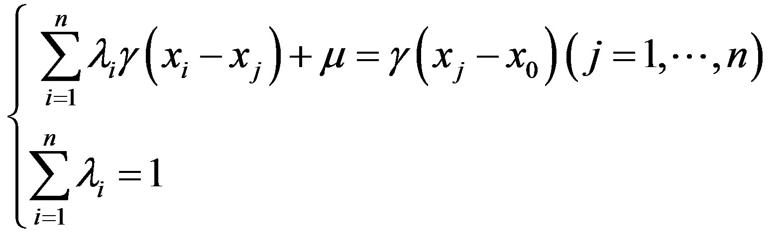 (4)
(4)
where  is the value of variogram between location
  and location
 . All weights
  and Lagrange multiplier
  can be calculated, and then
  can be obtained by (1).
2.2. Variogram
The key problem of Kriging is to determine the law of variable changed with space and then to estimate the unknown value based on the known samples. This law is variogram. Variogram is used to describe the spatial structure of variable.
The variogram of samples, which is also called experimental variogram, can be calculated by the following formula:
 (5)
(5)
where  is the number of pairs separated by vector
 , vector
  is lag distance,
  is the starting location and
  is the ending location. If
  is only dependent on the length of lag distance but not its direction,
  is isotropic, also the variable
  is isotropic. For the sake of simplicity, we only consider isotropy of Kriging.
Generally speaking, after the experimental variogram is computed by (5), we usually observe the distribution of variogram and then identify a reasonable variogram model. After that we use least square method to fit variogram in accordance with the principle of minimum variance estimate, which yields fitting curve called empirical variogram. Variogram model is usually a basic model or a linear combination of several basic models. The common theoretical model of variogram mainly includes linear model, spherical model, exponential model, Gaussian model and so on. Their mathematic expressions are as follows:
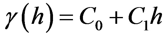
a) Linear model:
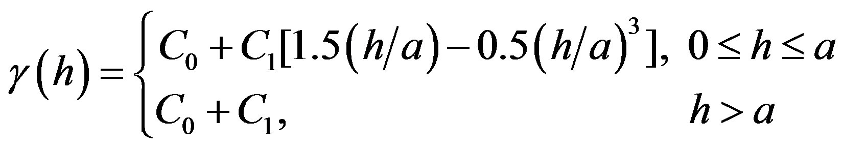
b) Spherical model:
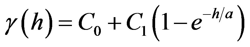
c) Exponential model:
d) Gaussian model:
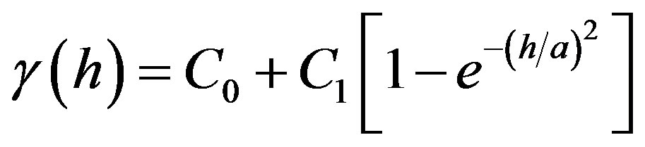
where  are unknown parameters that should be identified by least squares.
2.3. Existing Problem
At present, there are not very good methods to select the variogram models in general interpolation. In a general way, the reasonable variogram model is often identified based on the comparison of different variogram models. However, this method is time-consuming (because it need compute Kriging interpolation several times) and the types of variogram models are very finite, which make the variogram very difficult to describe the spatial distributional characteristics of true data .The general methods contain some subjectivity and arbitrariness. In order to overcome the existing problem, the least-square Support Vector Machine (LS-SVM) was introduced to fit the experimental variogram, and then the shortcoming of variogram model selection can be avoided. Based on least-square support vector machine, it does not need to identify the type of basic variogram models but to fit the experimental variogram according to its own distribution picture directly.
3. Least Squares Support Vector Machine
Support Vector Machines, as a novel learning machine developed by Vapnik and his coworkers in 1995 [2], have been introduced for pattern recognition and regression. Least squares support vector machine (LS-SVM), originally proposed by Suykens in 2001 [3], is one kind of SVM. LS-SVM transforms inequality constraints of standard SVM to equality constraints.
Given a training data set of samples,
 , where
  is the i-th input data. The LS-SVM approach aims at identify the parameters of the model:
 (6)
(6)
where  is weight vector,
  is a function which maps the input data into a higher dimensional feature space.
LS-SVM is to solve the following optimization problem:
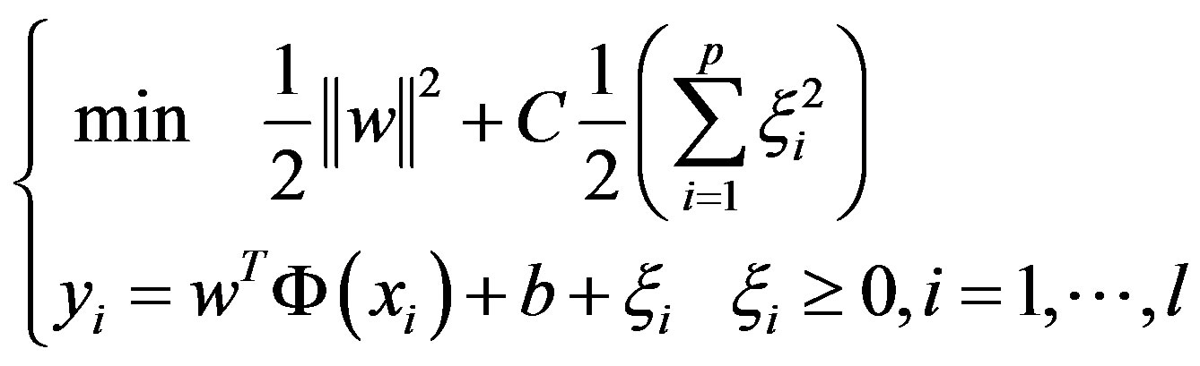 (7)
(7)
where  denotes regression error for sample
 ,
,  is a bias scalar, and
  is a given positive constant. After introducing Lagrangian multipliers
 , based on Karush-Kuhn-Tuchker conditions, we obtain the nonlinear function based on LS-SVM:
 (8)
(8)
where  is kernel function.
A Large number of imitation tests have shown that Radial Basis Function (RBF) kernel function is more effective than others as a whole, so we select RBF kernel as the kernel of LS-SVM.
 .
.
Note that  and
and  are two parameters. They can be optimized by Genetic Algorithms [4].
4. Support Vector Machine-Kriging Method
There are mainly three steps in SVM-Kriging method as follows:
1) Use (5) to compute experimental variogram  ;
;
2) Use LS-SVM with parameters optimized by Genetic Algorithm to fit the experimental variogram , and then get
 ;
;
3) Use (4) to get the weights  for every point
  and then obtain the estimated value
  at
at  by using (1).
5. Application in Oceanic Missing Data Recovery
In order to test the effect of improved Kriging based on LS-SVM, this paper takes data derived Global Ocean Data Assimilation System (GODAS) as the experimental data. GODAS is developed at National Centers for Environmental Prediction (NCEP) Centers, and GODAS data are time series of monthly average derived from GODAS operational datasets. The area coverage is [120.5˚E-71.5˚W, 60˚S-58˚N]. We selected four representative months January, April, July, and October of 2006 as test time, sea surface salinity (5 m deep in this paper) and the sea surface height relative to Geoid (sshg) as variables.
5.1. Interpolation Process
As the process of different months and different variables are similar, we take sshg in January 2006 as an example to introduce interpolation in detail and draw a compareson of different variogram model.The area coverage of sshg is [120.5˚E-71.5˚W, 60˚S-58˚N], and the spatial resolution is 2˚ × 2˚.The number of total grid points are 5100 (85 × 60), including a total of 4215 points in ocean availably. We selected 75% of them (3161) randomly as cross-validation data, and the remaining data (1054) are taken as known observed data. Figure 1 shows the remaining data after take out of 75% of available data.
Firstly, compute the experimental variogram. The experimental variogram was computed by (5) based on 1054 known data (Figure 2). Secondly, obtain empirical variogram. The empirical variogram was obtained by fitting based on different variogram models (Figure 3). At last, obtain the estimated values. Kriging interpolations

Figure 1. The remaining available sshg data.
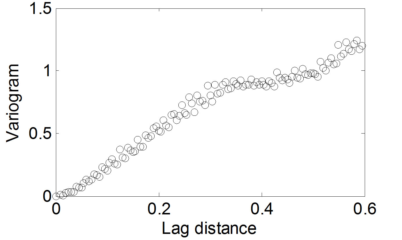
Figure 2. Experimental variogram.
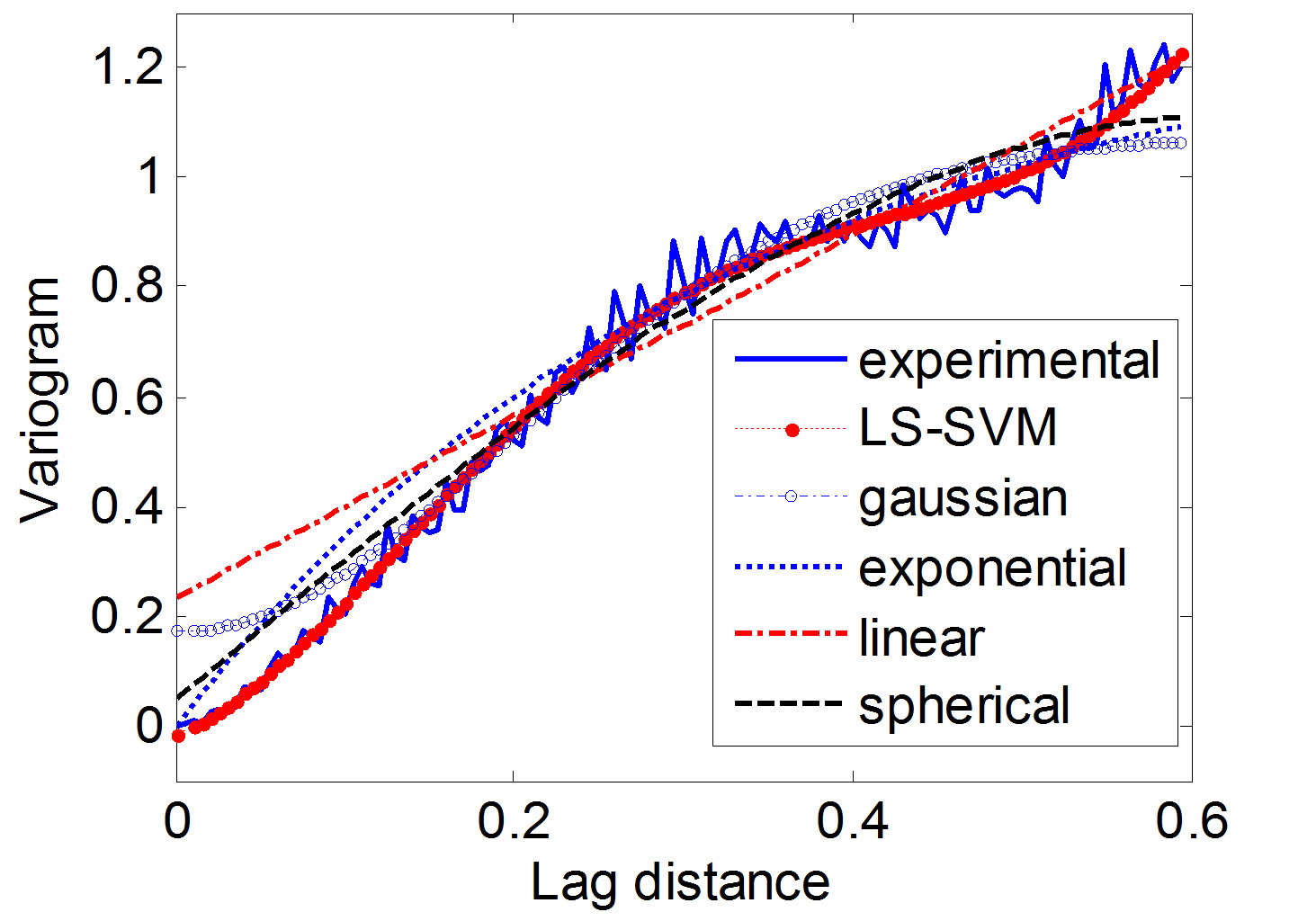
Figure 3. Experimental and different model variograms.
were carried out by using the obtained empirical variograms of different variogram models.
As the other interpolation processes of different months and variables are similar, the descriptions about them are omitted.
5.2. Cross-Validation Results
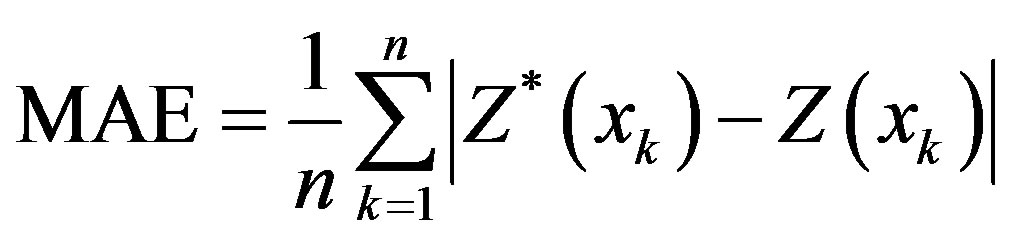
In order to analyze the interpolation quality, an evaluation by cross validation has been carried out. The cross validation starts by eliminating some available sample points randomly, the Kriging methods are then applied to estimate the missing value on basis of the remaining known sample points. The errors between estimated values and the observed values at missing points are calculated. The kinds of quantitative Error calculated mainly contain mean error (ME), mean absolute error (MAE), root mean square prediction error (RMSPE).The definitions of ME, MAE and RMSPE are as follows:
 (9)
(9)
 (10)
(10)
 (11)
(11)
RMSPE is a quantity used to compare the quality of different interpolation methods. RMSPE is smaller, the interpolation method is better. Based on differential variogram models, the Kriging interpolations with selected data are carried out. Following tables are error results of different months and different variables by cross-validation (See Table 1 and Table 2). The values with underline denote that they are minimal in their columns.
The error results have shown that the RMSPE of SVM-Kriging is smaller than others as a whole and the SVM-Kriging method is of adaptive advantage for real data of different variables at different time.
6. Conclusion
Kriging interpolated results are dependent on the selection of variogram model largely, and different variogram model will lead to different results. In this paper, the sea surface salinity and the sea surface height relative to Geoid are applied to test the interpolation effect. Tests have shown that the empirical variogram based on LS-SVM model improve the Kriging results by contrast with other variogram models, and it also avoids the subjectivity of selecting the type of basic variogram models. Therefore, the improved SVM-Kriging is a good and adaptive interpolation method for the real data, especially for the
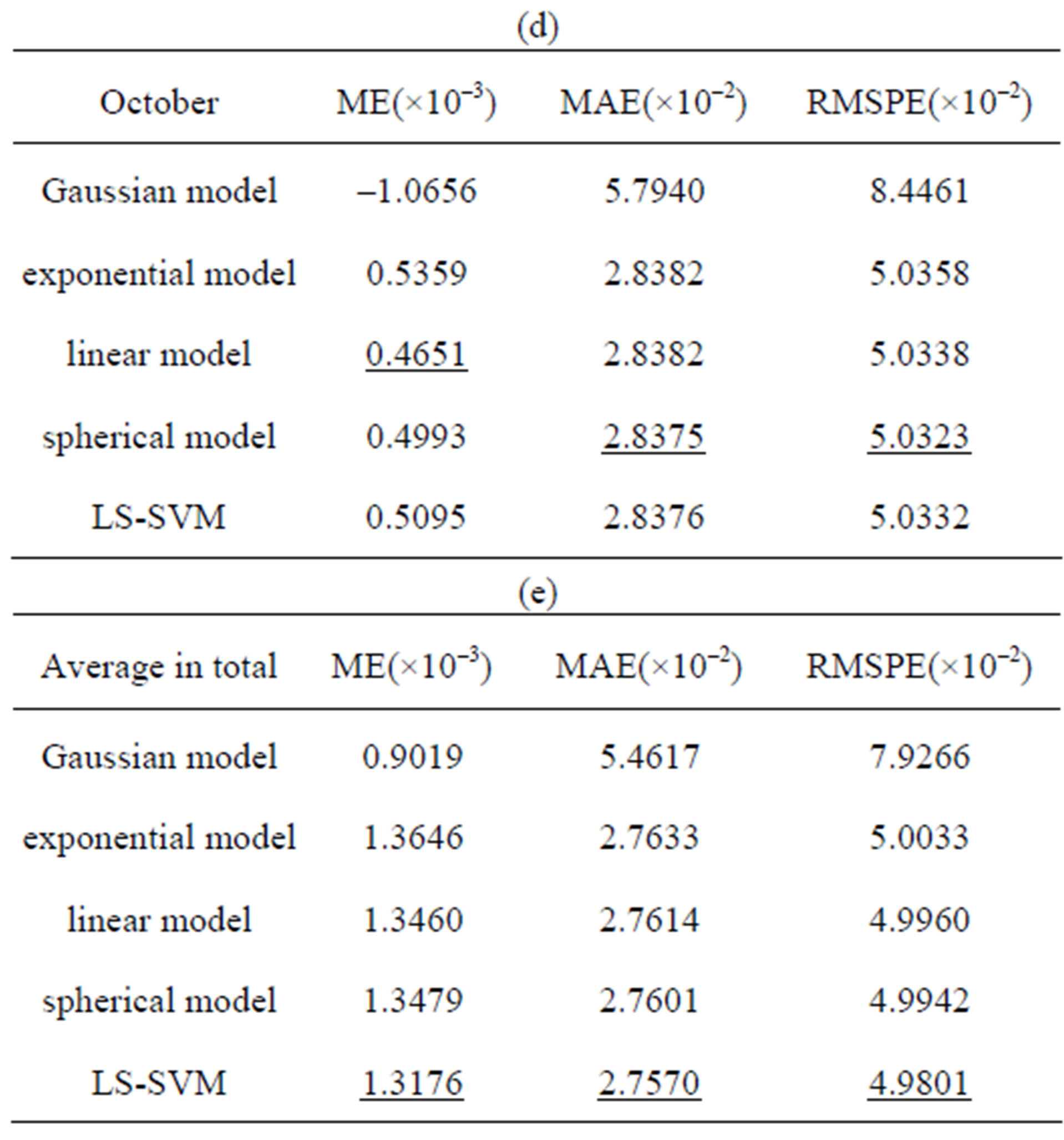
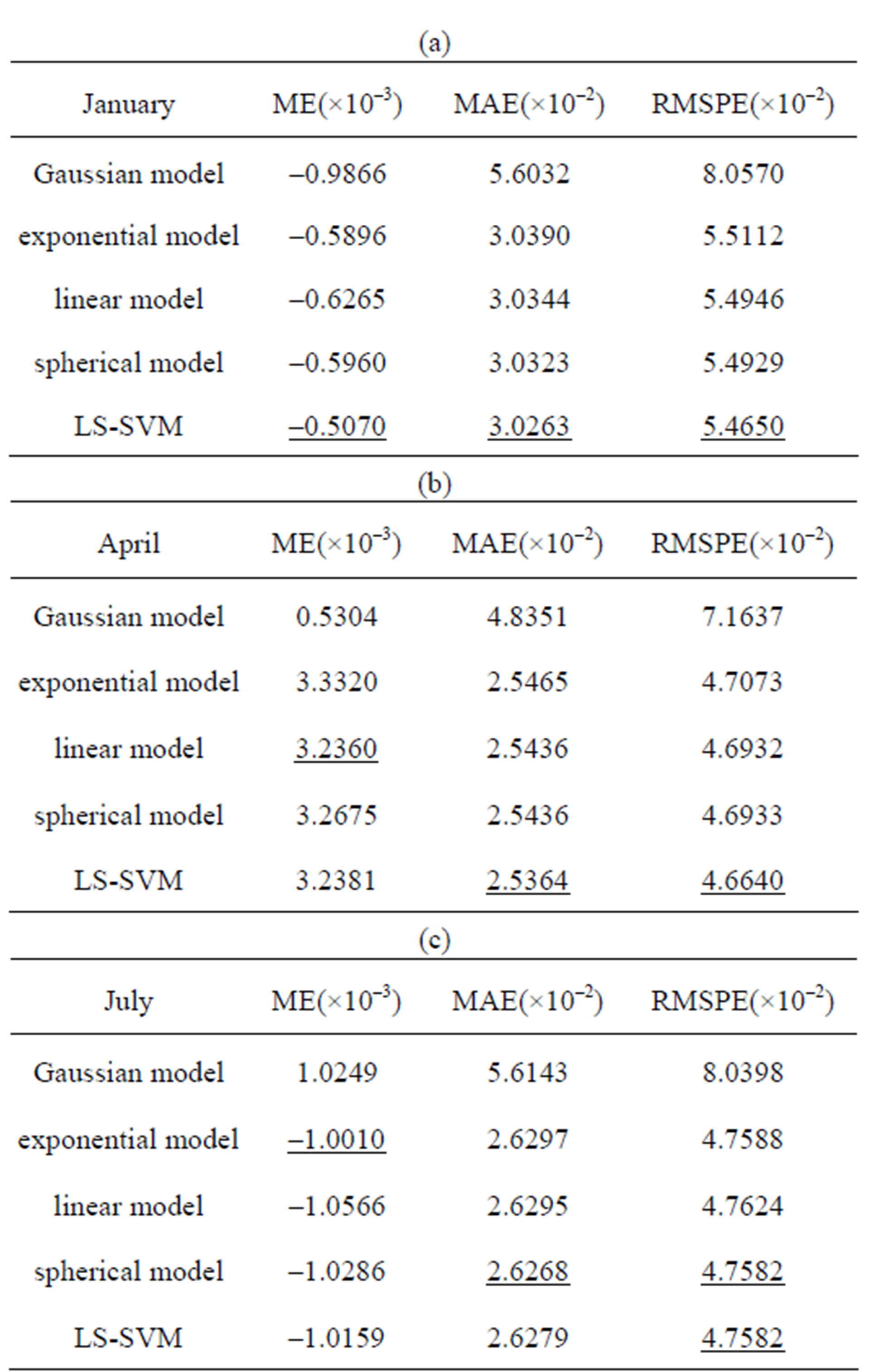
Table 1. The comparison of interpolation quality based on different variogram models to the sea surface height relative to Geoid (meter).


Table 2. The comparison of interpolation quality based on different variogram models to sea surface salinity (Kg/kg).
data containing complicated spatial structure
REFERENCES
- R. D. Zhang, “Spatial Variability Theory and Its Application,” Science Press, Beijing, 2005
- V. N. Vapnik, “The Nature of Statistical Learning Theory,” Springer-Verlag, New York, 1995.
- J. A. K. Suykens, J. Vannderwalle and B. D. Moor, “Optimal Control by Least Squares Support Vector Machine,” Neural Network, Vol. 14, No. 1, 2001, pp. 23-35. doi:10.1016/S0893-6080(00)00077-0
- K. F. Liu and R. Zhang, “Minimal Risk Based on the Structure of the Support Vector Machine Methods and Its Application in Numerical Forecast Optimization of Subtropical High,” Journal of Basic Science and Engineering, Vol. 14, No. 3, 2006, pp. 384-389.
NOTES
*Project supported by the National Natural Science Foundation of China (No. 41276036).