Int'l J. of Communications, Network and System Sciences
Vol.1 No.3(2008), Article ID:116,8 pages DOI:10.4236/ijcns.2008.13030
Relations among Mobility Metrics in Wireless Networks
Computing and Information Science, University of Guelph, Canada
E-mail: {xshu, xli}@uoguelph.ca
Received on June 1, 2008; revised and accepted on August 29, 2008
Keywords:Mobility Metrics, Link Failure Rate, Simulation
Abstract
In wireless network simulation analysis, researchers tweak mobility metrics, such as the speed or the pause time of the nodes, to get different stability levels of the network. Meanwhile, in theoretical analysis, link failure rate is widely used to model the stability of a wireless network. This paper presents an analysis of a simplified mobility model and shows that the link failure rate is positively correlated with the average speed of nodes in this model. Though this result is based on a mobility model with many restrictions, a simulation evaluation suggests that the result still holds in the popular random waypoint model and random direction model. Based on this observation, this paper also encourages the use of link failure rate as mobility metric instead of the problematic pause time in future practice.
1.Introduction
In simulation analysis of wireless networks, the movement of virtual nodes follows certain patterns called mobility models. The best known and widely used mobility model is the random waypoint model in which each host alternately pauses for a random length of time and moves to a new location at a random speed [1]. Recent research has focused a lot of attention on other models, such as the random direction model [2], random trip model [3] and empirically-based models [4]. Whatever the mobility model used in a simulation, in general, if nodes pause shorter or move faster, two nearby nodes will have a higher probability of moving out of the radio range of each other and the topology of wireless networks will be more unstable. The pause time and the speed of nodes are widely used as mobility metrics to measure the stability of a wireless network in simulation analysis.
Differing from simulation studies, theoretical analysis jumps to modeling the stability of wireless links directly, as they are easier to handle mathematically. It is common in theoretical analysis to make assumptions that the lifetime of links follows a probability distribution, such as the exponential distribution [5]. Generally, the shorter the average link lifetime is, or the more links fail in a unit of time, the more unstable a wireless network will be.
Both simulation and theoretical analysis can provide valuable information about the characteristics of a wireless network. However, the mobility models and mobility metrics used in these two methods are different; thus, the results produced by them are not directly comparable. This paper presents an analysis of a simplified mobility model and shows that the link failure rate is positively correlated with the average speed of nodes in this model. This result creates a mathematical bridge between these two analysis methods, and suggests that average speed is a better mobility metric than the widely used pause time as it is linear with link failure rate. Although we obtain this conclusion under a mobility model with strict restrictions, a simulation evaluation suggests that the analysis result still holds in the popular random waypoint model and random direction model.
The remainder of this paper is organized as follows. Section 2 outlines related work. Section 3 presents the mathematical relation between link failure rate and node speed. Section 4 analyzes the properties of mobility metrics. In Section 5, we conclude this paper and address some ideas about future research.
2.Related Work
The most popular mobility model, the random waypoint model, was first used by Johnson and Maltz in the evaluation of the Dynamic Source Routing (DSR) protocol [1,6]. It is implemented in the simulation tools ns-2 [7] and GloMoSim [8] and widely used in evaluations of network algorithms and protocols. In a typical simulation with random waypoint model, N nodes are placed at random initial locations over a rectangular area of size Xmax × Ymin. Each node is then assigned a destination which is uniformly distributed over the two-dimensional area with a speed v, which is either in the form of a constant value or in the form of a certain distribution [1,9,10], such as uniform distribution over (0, Vmax]. A node will then start travelling toward the destination on a straight line, at the chosen speed v. Upon reaching the destination, the node stays there for some constant or random pause time. When pause time expires, it chooses the next destination and speed in the same way, and the process repeats until the simulation ends.
The original random waypoint model is problematic. It has been observed in [11,12] that the spatial distribution of nodes tends to be denser at the center of the rectangular simulation area as the simulation runs. Bettstetter et al. presented a solution to the spatial distribution changing problem by setting up a proper initial distribution of nodes [13]. Another problem is that average speed of nodes decreases gradually as more and more nodes become“stuck” travelling long distances at low speeds [14]. In particular, if the random speed is uniformly chosen from (0, Vmax], the average speed will decrease to 0 over time rather than the desired speed of Vmax/2. Thus, a “pre-run” to stabilize the random waypoint model is necessary. This paper applied such method to ensure the accuracy of the simulation.
Random direction model is another widely studied mobility model [11]. Its difference with the random waypoint model is that each node chooses a direction rather than a position as the next target. There are two variations, called random direction with wrap around [15] and random direction with reflection [16], representing two different strategies when a node hits boundary of simulation area. Random direction model is less physically appealing than random waypoint model. However, it exhibits some nice properties, especially useful in theoretical studies; because, at any time of simulation, users are uniformly distributed within the space and distributions of speeds are easily calculated and understood with respect to the model inputs [2].
Theoretical analysis usually does not discuss the movement of nodes, but abstracts wireless networks to link level. For example, Nasipuri and Das assumed that the lifetime of a wireless link between a pair of nodes is a random variable independent from other links, and it is exponentially distributed with mean , which means that the probability distribution function is
  [5]. The advantage of this assumption is its simplicity, that is, in any given time unit, the same proportion of nodes will depart from the radio range of current node. Tsirigos et al. [17] proposed an analytic model which is based on the assumption of the lifetime of routes rather than links, but their analysis methods are similar.
To see how a protocol performs in wireless networks with different stability levels, researchers evaluate metrics under several simulations with different node mobility setups. In the paper presenting DSR, which is also the first paper to use the random way point model [1], Johnson simulated several situations with different node pause times, and compared how metrics, such as the packet delivery ratio and routing overhead, change over increasing pause time. Later, many researchers followed Johnson’s method and used pause time rather than speed as a control variable of mobility in their protocol performance comparison researches [9,10].
Johansson et al. used the overall average speed of nodes as the mobility metric in a simulation [18]. They suggested that the pause time metric is ill-defined when node motion is continuous or when nodes use different pause times; however, the speed is more relevant for how often links break down and form. A paper by Perkins et al. also supports using speed as a metric by showing that: although both node speed and pause time can affect the performance of routing protocols, node speed is shown to be a significant factor, while pause time is not [19]. Camp and Boleng showed that the relation between node speed and link breakage is linear with simulation results [20,21]. This observation is confirmed by later researches [22,23].
3.Link Failure Rate and Speed
For simplicity and clarity of our illustration, we will analyze a simplified version of the random waypoint model with the following assumptions:
♦ Nodes move in an arbitrarily large area without obstacles.
♦ Pause time is zero-nodes are always moving toward their destination.
♦ All nodes move at the same speed v0.
Such simplifying assumptions help to isolate and emphasize how the motion of nodes affects the lifetime of links. Moreover, simulation evaluation in the latter part of this section shows that our conclusion based on this model remains true for the original random waypoint model or random direction model.
3.1.Analysis of Link Failure Rate
In the simplified mobility model, all nodes have same circle radio range with radius R. Therefore, a bidirectional link is created when the distance of two nodes is less than R, and it is broken when the distance is larger than R. The time interval, T, between the creation and the loss of the link is a random variable called the lifetime of the link. From another aspect, an established
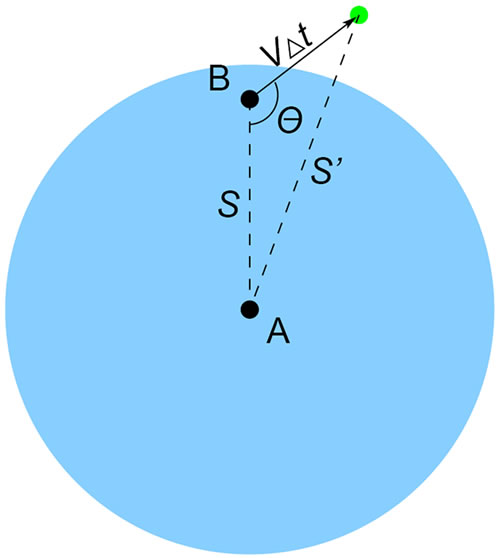
Figure 1. Illustration of Theorem 2.
link may have a probability λt to fail at time t, which can be defined formally as:
Definition 1: Link lifetime T is a random variable. For any time t and a very small time interval Δt, if the conditional probability P[T < t + Δt|T ≥ t] = λtΔt + o(Δt), we say that λt is the link failure rate at time t.
By this definition, it is not hard to see that if the link failure rate λ is constant, the probability distribution function of link lifetime is exponential. This implies that the constant link failure rate model and exponentially distributed model are identical in theoretical analysis. Meanwhile, if λ is constant, how long the link already lasts does not affect the future status. This stateless property is very nice for theoretical analysis.
Now, with the formal definition of link failure rate, we can prove following theorem:
Theorem 2: Suppose at time t, the relative speed of two nodes forming a link is random variable V. Then the failure rate of this link is .
.
Proof: Let A and B be two mobile nodes. Assume that at time t, the distance of A and B is random variable S, and the angle between the directions of relative speed and the straight line connecting the two nodes is random variable Θ. Since node B is uniformly distributed in the circle radio range of node A as indicated in Figure 1, the probability distribution function of S is:
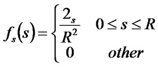 (1)
(1)
And Θ is uniformly distributed on [0,2π), so its probability function is:
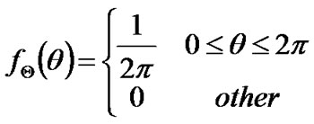 (2)
(2)
By the law of cosine, after a small interval Δt, the distance of the two nodes will be as follows at time t+Δt:

Let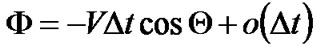 , and let its probability distribution function (PDF) be fФ. As Δt is sufficiently small and the relative speed is a limited number, there exists a constant C, such that φM = CΔt and |Ф| ≤ φM.
Since S' = S + Ф, by the convolution law, the PDF of S' is:

If the lifetime random variable of the link is T, and the link has existed for time t0, we will have:
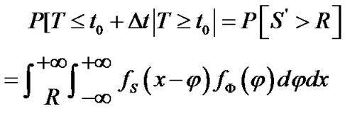 (3)
(3)
By Equation 1,  when
when  and
and ; thus,
  is not zero if
 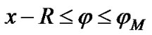 and
and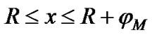 . Therefore, Equation 3 can be written as:
 (4)
(4)
In above equation, 0 ≤ φ ≤ φM = CΔt, thus:
 (5)
(5)
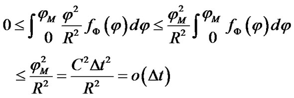
With this result, Equation 3 can be simplified as:
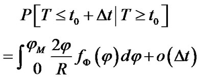 (6)
(6)
As Ф = ?VΔt cosΘ + o(Δt), where V and Θ are two independent random variables, so the conditional mathematical expectation of Ф is:
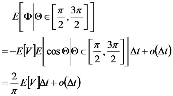
Furthermore, by the definition of mathematical expectation,
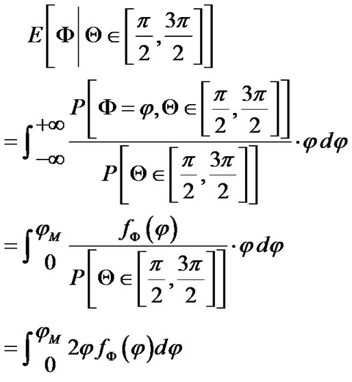
Therefore:
 (7)
(7)
Combining Equation 6 and Equation 7, we get:
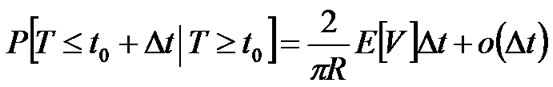
Thus, by Definition 1, the failure rate of this link is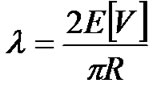 .
.
From Theorem 2 we can see that link failure rate is positively correlated with the mathematical expectation of relative speed. This conclusion coincides with the intuition that if nodes move faster, links will have higher probability to break. Also, Theorem 2 shows that the link failure rate is inversely correlated with the radius of the radio circle. Larger radio range makes link more stable, that is, the probability of a node moving out of the current node’s radio range is smaller.
Until now, we have not used the third assumption of simplified mobility model, that is, all nodes move at a constant speed v0. With this assumption, we can prove a simplified version of Theorem 2:
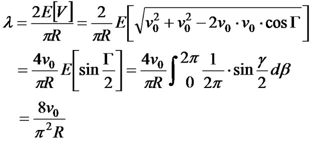
Corollary 3: Suppose that all nodes move at a constant speed, v0, and г is the random variable of angle between moving directions of two nodes, which are uniformly distributed on [0, 2π). Then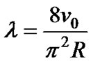 .
.
Proof: By Theorem 2 and the law of cosine,
3.2.Simulation
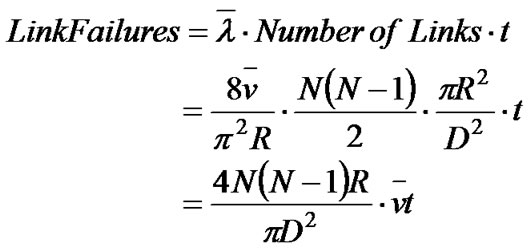
By Corollary 3, assuming that all nodes in a simulation move at the overall average speed , we can estimate the average link failure rate as:

So, if a simulation has N nodes moving in a D×D rectangular area, the number of link failures during time t is approximately equal to:
Ten separate simulations were conducted to study the accuracy of the above prediction for each mobility model. Each simulation contains 100 nodes moving in a 1000m×1000m rectangular area at uniformly distributed speeds over [Vm, 2Vm], where Vm is selected from 1m/s to 10m/s.
In the random waypoint model, to avoid the spatial distribution change problem [13] and speed dropping problem [14], every simulation is given a 1000-second pre-run period to warm-up the mobility model to a stable state, and only the data collected from after the 1000-second period is used. Since the speed of nodes is uniformly distributed, the expected average speed of random waypoint model is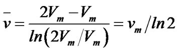 .
.
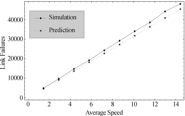
Figure 2(a) illustrates that the predicted number of link failures is close to the actual number in the random waypoint model simulation. Although the random waypoint model has boundaries, which is different from the simplified model, the density of nodes is higher
 (a)
(a)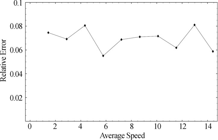 (b)
(b)
Figure 2. Relation of link failure rate with average speed in random waypoint model (speed= [v,2v], pause=0s, area= 1000m * 1000m).
 (a)
(a) (b)
(b)
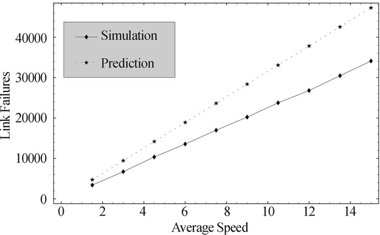
Figure 3. Relation of link failure rate with average speed in random direction model with reflection (speed= [v,2v], pause= 0s, area=1000m * 1000m).
around the center, so the nodes near the borders will not significantly impact the result. Figure 2(b) shows that the relative error of our prediction is 5% to 8%, which is a small range and it approximates to a horizontal line. It means that our prediction is increasing at the same ratio with the actual number of link failures, or in other words, the actual number is linear with our prediction and the average speed. Therefore, to get a more accurate result, we can simply multiply an empirical constant to the predicted number.
Different from the random waypoint model, nodes in the random direction model are always distributed uniformly in the simulation area. Figures 3 and 4 show the data collected from the random direction model with reflection [16] and random direction model with wrap around [15] with the same simulation settings as random waypoint model. Similar to the previous result, the linear property holds in these two models as well; and the relative error is small and can be fixed with an empirical constant.
The reason why predictions overestimate the results in the random direction model simulation with reflection while underestimate in the other two lays behind radio range distortion problem caused by the borders of simulation area. Figure 5 illustrates the shape of the radio range of node A when it is not far away from the border. By the nature of random direction model with reflection, if node B, which is in the radio range of A, is right next to the border of the simulation area, it could not possibly escape from A in the next unit of time. However, this is possible in the random direction model with wrap around.
In general, the ratio of the girth of radio covered area to the size of the area is a decisive factor of the frequency of link breakages, since with the same size of radio area, the longer the girth is, the more nodes could possibly move in and out from the area. It is not hard to see from Figure 5 that the girth/area ratio of the random direction model with reflection is smaller than the ratio of simplified model whose radio range is always a circle. The random direction model with wrap around has larger girth/area ratio than both of them. This characteristic causes the predictions, which are based on simplified model, overestimate the results in one model and underestimate in the other. The random way point model has similar radio range distortion problem with the random direction model with reflection. However, since there are few nodes close to the border in this model [14], the problem will not affect the prediction results as much.
 (a)
(a)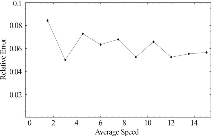 (b)
(b)
Figure 4. Relation of link failure rate with average speed in random waypoint model with wrap around (speed= [v,2v], pause=0s, area= 1000m * 1000m).
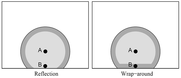
Figure 5. Radio range of a node near the border in the random direction model. The gray area is radio range of the node and the dark gray area is where a node in the radio range could possibly escape in the next unit of time.
4.Mobility Metrics
Mobility metrics is a measure of how actively nodes move in a simulation. With different mobility metrics setups, researchers can produce different scenarios to evaluate the performance of their wireless network protocols. One of the most popular mobility metrics is pause time. In the paper presenting DSR [1], Johnson simulated several situations with different node pause times, and compared how performance metrics, such as packet delivery ratio and routing overhead, change over the increasing pause time. Johansson used average speed of nodes as mobility metric in his simulation study [18].
Link failure rate, which reflects the wireless network topology change rate, can be used for mobility metrics as well. Usually, we cannot set link failure rate directly in wireless network simulations; however, as we presented in Section 3, link failure rate is positively correlated with the average speed of nodes. Therefore, we can create any level of link failure rate as we want with proper setup of the speed of nodes and the radio range. The remainder of this section presents an analysis of the mathematical relationship between the link failure rate and the other two mobility metrics.
Suppose in a random waypoint model simulation, a node moves at constant speed v and stays at each destination for a constant pause time, p. Let δ be the average distance between two waypoints. If the node passed through n destination points, and n is large enough, which implies that this simulation has been run long enough, it can be estimated that the overall average speed of the nodes as follows:

This formula shows that the pause time p is not linear with the average speed, and obviously, it is not linear with the link failure rate as well, since average speed is linear with link failure rate. The derivative of the average speed is:
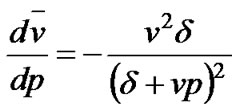
This implies that the change of p has a larger impact on the expectation of average speed and the link failure rate when pause time, p, is comparatively small. However, when p is large, its impact is not that distinct. If one uses pause time as the X-axis of the graph showing how other network performance metrics change, the amplitude of these metrics will become smaller as pause time increases. This phenomenon, which has been observed in previous research [19], suggests that graph analysis with pause time as mobility metrics may be inaccurate and not intuitive.
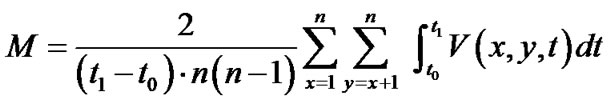
Johansson [18] defined another mobility metric as follows:
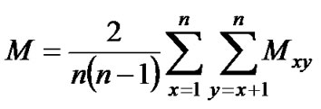
where n is the number of nodes, and Mxy is defined as the average relative speed between nodes x, y during the simulation. This mobility metric has a nice property-it is linear with the link failure rate.
Theorem 4: Let M be the mobility metric defined in[18] and  be the average link failure rate, then
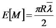 .
.
Proof: By Theorem 2, the failure rate of the link between x and y is 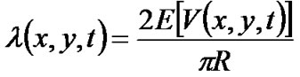 at time t, so
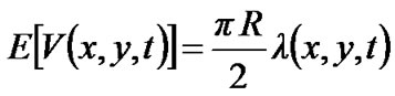 .
.
By the definition of M,
Therefore, its mathematical expectation is:
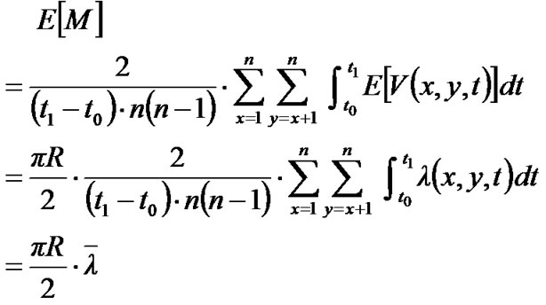
Since M is linear with link failure rate, it is more reasonable to use it as a mobility metric than pause time. However, Theorem 4 also shows a problem of this mobility metric. Consider two similar simulations, whereby nodes move at exactly the same speed and path. Suppose the first simulation has a larger radius of radio range. Although M shows no difference of the mobility levels of these two simulations, it is obvious that links in the second simulation are not as stable as in the first one since their radio range is smaller, and these two simulations will produce different analysis results. Therefore, the mobility metric should consider the radius R of radio range as well. By Theorem 4, if the mobility metric is defined as , the simulation analysis could avoid said situation. Or, the average link failure rate
  can be used as the mobility metric directly, since it has the same linear property as M and will not affect by the radius problem.
5.Conclusions and Future Work
By analyzing a simplified mobility model, which is similar to random waypoint model but has no boundary and no pause time, we find that the link failure rate is linear with the speed of nodes in simulation analysis. That is, if node increases speed, the number of links failing during a unit of time increases accordingly. This property makes average speed a better mobility metric than pause time, since it reflects the topology change rate better. Although this analysis is based on simplifying assumptions, simulation analysis suggests that the result can also be applied on the random waypoint and random direction models.
For future research, we believe that the study of link lifetime will be a great help for optimizing routing protocols, because a node can choose the appropriate link that has highest probability of living if it knows how link lifetime distributed. Bettstetter et al. have done a valuable job of analyzing the link lifetime of the random waypoint model [24]. We expect further study of link lifetime in real scenario based mobility model.
Based on this paper, we also conjecture that if two mobility models create the same probability distribution of link lifetime, a non-geographic-based wireless network algorithm should produce similar results on both mobility models. This implies that the link failure rate has great weight on the topological change of a wireless network.
6.References
[1] D. B. Johnson and D. A. Maltz,"Dynamic source routing in ad hoc wireless networks,"Mobile Computing, Chapter 5, pp. 153-181, 1996.
[2] P. Nain, D. Towsley, B. Liu, and Z. Liu," Properties of random direction models,"INRIA technical report RR-5284, July 2004.
[3] J. Y. Le Boudec and M. Vojnovic",Rerfect simulation and stationarity of a class of mobility models,"IEEE Infocom 2005, Miami, FL, 2005.
[4] A. K. Saha and D. B. Johnson, "Modeling mobility of vehicular ad hoc networks,"ACM VANET 2004, October 2004.
[5] A. Nasipuri and S. R. Das, "On-demand multipath routing for mobile ad hoc networks,"Proceedings of the 9th International Conference on Computer Communications and Networks (IC3N), Boston, October 1999.
[6] D. B. Johnson, D. A. Maltz, and J. Broch,"DSR: The dynamic source routing protocol for multi-hop wireless ad hoc networks,"Ad Hoc Networking, edited by Charles E. Perkins, Addison-Wesley, Chapter 5, pp. 139-172, 2001.
[7] The Network Simulator - ns-2, Online:http:// www.isi.edu/ nsnam/ns/, November 2006.
[8] Global Mobile Information System Simulation Library ?GloMoSim, ,November 2006, Online:
http://pcl.cs.ucla.edu/projects/glomosim/.
[9] J. Broch, D. A. Maltz, D. B. Johnson, Y. C. Hu, and J. Jetcheva," A performance comparison of multi-hop wireless ad hoc network routing protocols,"Mobile Computing and Networking (MobiCom), pp. 85-97, 1998.
[10] C. E. Perkins, E. M. Royer, S. R. Das, and M. K. Marina, "Performance comparison of two on-demand routing protocols for ad hoc Networks,"IEEE personal Communications, Vol. 9, No. 1, pp. 16-28, February 2001.
[11] C. Bettstetter, "Mobility modeling in wireless networks: Categorization, smooth movement, and border effects,"ACM Mobile Computing and Communications Review, Vol. 5, No. 3, 2001.
[12] E. M. Royer, P. M. Melliar-Smith, and L. E. Moser,"An analysis of the optimum node density for ad hoc mobile networks,"Proceedings of IEEE International Conference on Communications (ICC), June 2001.
[13] C. Bettstetter, G. Resta, and P. Santi," The node distribution of the random waypoint mobility model for wireless ad hoc networks,"IEEE Transactions on Mobile Computing, Vol. 02, No. 3, pp. 257-269, July-September 2003.
[14] J. Yoon, M. Liu, and B. Noble, Random waypoint considered harmful,"IEEE Infocom 2003, San Francisco, CA.
[15] Z. J. Haas,"The routing algorithm for the reconfigurable wireless networks,"Proceedings of ICUPC?7, San Diego, CA, October 1997.
[16] N. Bansal and Z. Liu, "Capacity, delay, and mobility in wireless ad-hoc networks,"Proceedings of INFOCOM 2003, San Francisco, CA, March 2003.
[17] A. Tsirigos, Z. J. Haas, and S. Tabrizi, "Multipath routing in mobile ad hoc networks or how to route in the presence of topological changes,"Proceedings of the MILCOM 2001 IEEE Military Communications Conference, October 2001.
[18] P. Johansson, T. Larsson, N. Hedman, B. Mielczarek, and M. Degermark, "Scenario-based performance analysis of routing protocols for mobile ad hoc networks,"Annual International Conference on Mobile Computing and Networking (MOBICOM), pp. 195-206, August 1999.
[19] D. D. Perkins, H. D. Hughes, and C. B. Owen,"Factors affecting the performance of ad hoc networks,"Proceedings of the IEEE International Conference on Communications (ICC), 2002.
[20] J. Boleng, "Normalizing mobility characteristics and enabling adaptive protocols for ad hoc networks,"LANMAN 2001: 11th, IEEE Workshop on Local and Metropolitan Area Networks, pp. 9-12, March 2001.
[21] T. Camp, J. Boleng, and V. Davies, "A survey of mobility models for ad hoc network research,"Wireless Communications F4 Mobile Computing (WCMC): Special Issue on Mobile Ad Hoc Networking: Research, Trends and Applications, 2002.
[22] L. Qin and T. Kunz, "Mobility metrics to enable adaptive routing in MANET,"Proceedings of the 2nd IEEE International Conference on Wireless and Mobile Computing, Networking and Communications (WiMob 2006), Montreal, Canada, pp. 1-8, June 2006.
[23] C. Yawut, B. Paillassa, and R. Dhaou, "Mobility metrics evaluation for self-adaptive protocols,"Journal of Networks, Academy Publisher, Finland, Vol. 3, No. 1, ISSN : 1796-2056, pp. 5364, January 2008.
[24] C. Bettstetter, H. Hartenstein, and X. Péez-Costa, "Stochastic properties of the random waypoint mobility model,"ACM/Kluwer Wireless Networks: Special Issue on Modeling and Analysis of Mobile Networks, 10(5), September 2004.