 Journal of Applied Mathematics and Physics, 2016, 4, 1585-1591 Published Online August 2016 in SciRes. http://www.scirp.org/journal/jamp http://dx.doi.org/10.4236/jamp.2016.48168 How to cite this paper: Haji, A., Keyim, T. and Yunus, B. (2016) Existence and Uniqueness of the Dynamic Solution of a Se- ries-Parallel Repairable System Consisting of Three-Unit with Multiple Vacations of a Repairman. Journal of Applied Mathe- matics and Physics, 4, 1585-1591. http://dx.doi.org/10.4236/jamp.2016.48168 Existence and Uniqueness of the Dynamic Solution of a Series-Parallel Repairable System Consisting of Three-Unit with Multiple Vacations of a Repairman Abdukerim Haji 1 , Tursunjan Keyim 1 , Bilikiz Yunus 2 1 College of Mathematics and System Sciences, Xinjiang University, Urumqi, China 2 College of Mechanical Engineering, Xinjiang University, Urumqi, China Received 17 March 2016; accepted 17 August 2016; published 24 August 2016 Abstract We investigate a series-parallel repairable system consisting of three-unit with multiple vacations of a repairman. By using -semigroup theory of linear operators in the functional analysis, we prove that the system is well-posed and has a unique positive dynamic solution. Keywords Series-Parallel Repairable System, -Semigroup, Dynamic Solution 1. Introduction The series-parallel repairable systems consisting of three-unit are frequently used in practice. Since the strong practical background of the series-parallel repairable systems consisting of three-unitrepairable system, many researchers have studied them extensively under varying assumptions on the failures and repairs, see [1] [2]. Repairman is one of the essential parts of repairable system, and can affect the economic benefit of the system. The repairman leaves for a vacation when there are no failed units for repair in system, which can have impor- tant influence to performance of system. In [3], the authors studied series-parallel repairable system consisting of three-unit with multiple vacations of a repairman and obtained some reliability expressions such as the Lap- lace transform of the reliability, the mean time to the first failure, the availability and the failure frequency of the system. In [3], the authors used the dynamic solution in calculating the availability and the reliability. But they did not discuss the existence of the positive dynamic solution. Motivated by this, we study in this paper the well- posedness and the existence of a unique positive dynamic solution of the system, by using 0 -semigroup theory of linear operators. The series-parallel repairable system consisting of three-unit with multiple vacations of a repairman can be described by the following equations (see [3]). 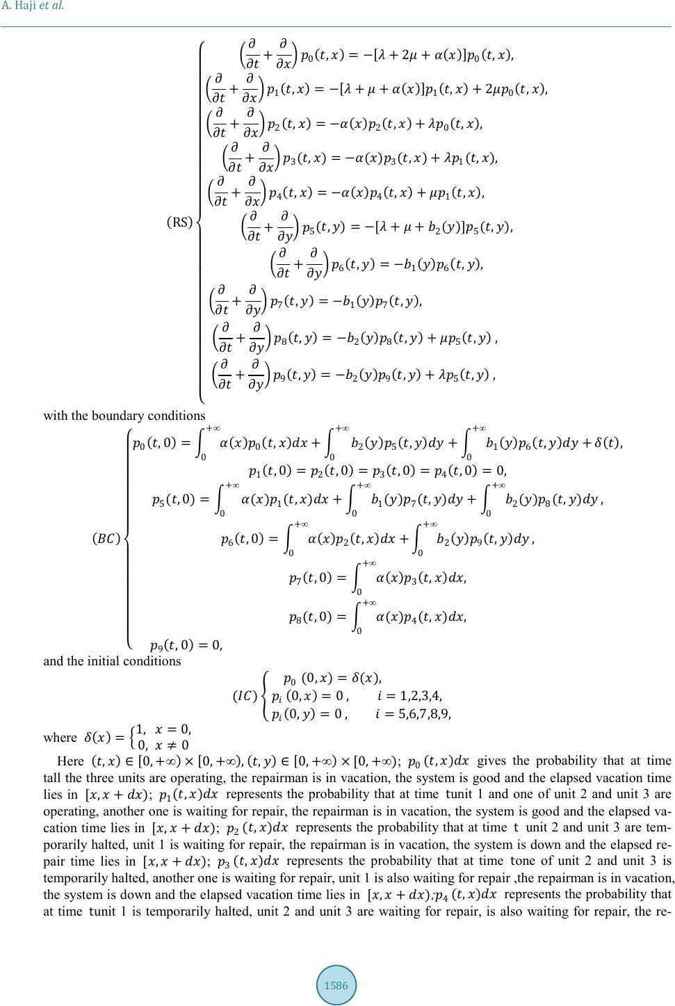 A. Haji et al. ( RS ) + 0 ( , ) = [ + 2+ ( ) ] 0 ( , ) , + 1 ( , ) = [ + + ( ) ] 1 ( , ) + 2 0 ( , ) , + 2 ( , ) = ( ) 2 ( , ) + 0 ( , ) , + 3 ( , ) = ( ) 3 ( , ) + 1 ( , ) , + 4 ( , ) = ( ) 4 ( , ) + 1 ( , ) , + 5 ( , ) = [ + + 2 ( ) ] 5 ( , ) , + 6 ( , ) = 1 ( ) 6 ( , ) , + 7 ( , ) = 1 ( ) 7 ( , ) , + 8 ( , ) = 2 ( ) 8 ( , ) + 5 ( , ) , + 9 ( , ) = 2 ( ) 9 ( , ) + 5 ( , ) , with the boundary conditions ( ) 0 ( ,0 ) = ( ) 0 ( , ) + +∞ 0 2 ( ) 5 ( , ) + 1 ( ) 6 ( , ) + +∞ 0 +∞ 0 ( ) , 1 ( ,0 ) = 2 ( ,0 ) = 3 ( ,0 ) = 4 ( ,0 ) =0, 5 ( ,0 ) = ( ) 1 ( , ) + 1 ( ) 7 ( , ) +∞ 0 +∞ 0 + 2 ( ) 8 ( , ) +∞ 0 , 6 ( ,0 ) = ( ) 2 ( , ) + +∞ 0 2 ( ) 9 ( , ) +∞ 0 , 7 ( ,0 ) = ( ) 3 ( , ) , +∞ 0 8 ( ,0 ) = ( ) 4 ( , ) , +∞ 0 9 ( ,0 ) =0, and the initial conditions ( ) 0 ( 0, ) = ( ) , ( 0, ) =0 ,=1,2,3,4, ( 0, ) =0 ,=5,6,7,8,9, where ( ) = 1, =0, 0,0 Here ( , ) [ 0,+∞ ) × [ 0,+∞ ) , ( , ) [ 0,+∞ ) × [0,+∞); 0 ( , ) gives the probability that at time tall the three units are operating, the repairman is in vacation, the system is good and the elapsed vacation time lies in [,+ ); 1 ( , ) represents the probability that at time tunit 1 and one of unit 2 and unit 3 are operating, another one is waiting for repair, the repairman is in vacation, the system is good and the elapsed va- cation time lies in [,+ ); 2 ( , ) represents the probability that at time t unit 2 and unit 3 are tem- porarily halted, unit 1 is waiting for repair, the repairman is in vacation, the system is down and the elapsed re- pair time lies in [,+ ); 3 ( , ) represents the probability that at time tone of unit 2 and unit 3 is temporarily halted, another one is waiting for repair, unit 1 is also waiting for repair ,the repairman is in vacation, the system is down and the elapsed vacation time lies in [,+ ); 4 ( , ) represents the probability that at time tunit 1 is temporarily halted, unit 2 and unit 3 are waiting for repair, is also waiting for repair, the re- 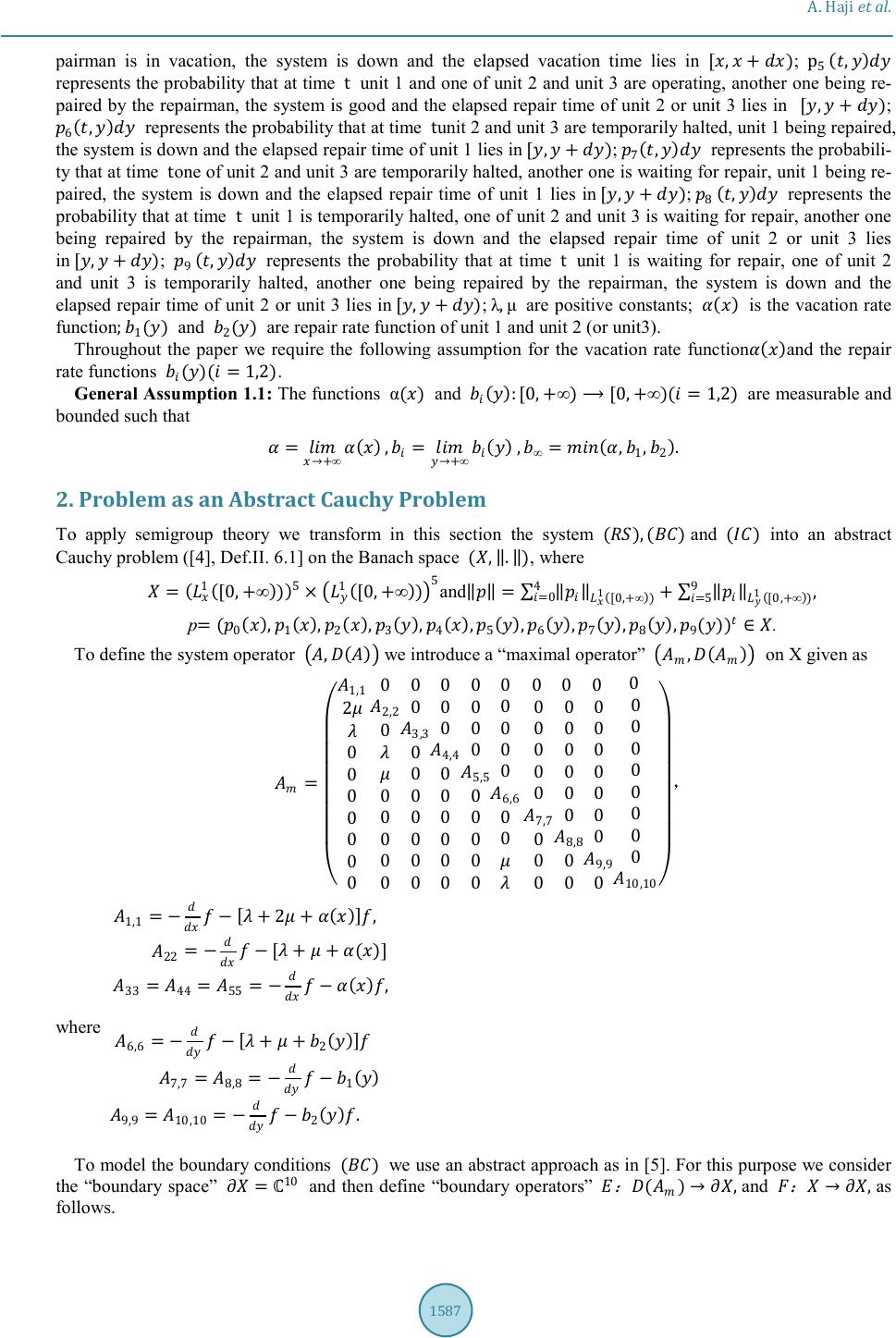 A. Haji et al. pairman is in vacation, the system is down and the elapsed vacation time lies in [,+ ); p 5 ( , ) represents the probability that at time t unit 1 and one of unit 2 and unit 3 are operating, another one being re- paired by the repairman, the system is good and the elapsed repair time of unit 2 or unit 3 lies in [,+); 6 ( , ) represents the probability that at time tunit 2 and unit 3 are temporarily halted, unit 1 being repaired, the system is down and the elapsed repair time of unit 1 lies in [,+ ); 7 ( , ) represents the probabili- ty that at time tone of unit 2 and unit 3 are temporarily halted, another one is waiting for repair, unit 1 being re- paired, the system is down and the elapsed repair time of unit 1 lies in [,+ ); 8 ( , ) represents the probability that at time t unit 1 is temporarily halted, one of unit 2 and unit 3 is waiting for repair, another one being repaired by the repairman, the system is down and the elapsed repair time of unit 2 or unit 3 lies in [,+ ); 9 ( , ) represents the probability that at time t unit 1 is waiting for repair, one of unit 2 and unit 3 is temporarily halted, another one being repaired by the repairman, the system is down and the elapsed repair time of unit 2 or unit 3 lies in [,+ ); λ,μ are positive constants; ( ) is the vacation rate function; 1 () and 2 () are repair rate function of unit 1 and unit 2 (or unit3). Throughout the paper we require the following assumption for the vacation rate function ( ) and the repair rate functions ()(=1,2). General Assumption 1.1: The functions α() and ( ) :[0,+∞)[0,+∞)(=1,2) are measurable and bounded such that = +∞ ( ) , = +∞ ( ) , ∞ = ( , 1 , 2 ) . 2. Problem as an Abstract Cauchy Problem To apply semigroup theory we transform in this section the system ( ) , ( ) and () into an abstract Cauchy problem ([4], Def.II. 6.1] on the Banach space (, . ), where = ( 1 ( [0,+∞ ) ) ) 5 × 1 ( [0,+∞ ) ) 5 and = 1 ( [0,+∞ ) ) + 1 ( [0,+∞ ) ) , 9 =5 4 =0 p=( 0 ( ) , 1 ( ) , 2 ( ) , 3 ( ) , 4 ( ) , 5 ( ) , 6 ( ) , 7 ( ) , 8 ( ) , 9 ()) . To define the system operator , ( ) we introduce a “maximal operator” , ( ) on X given as = 1,1 2 0 0 0 0 0 0 0 0 2,2 0 0 0 0 0 0 0 0 3,3 0 0 0 0 0 0 0 0 0 0 4,4 0 0 0 0 0 0 0 0 0 0 5,5 0 0 0 0 0 0 0 0 0 0 6,6 0 0 0 0 0 0 0 0 7,7 0 0 0 0 0 0 0 0 0 0 8,8 0 0 0 0 0 0 0 0 0 0 9,9 0 0 0 0 0 0 0 0 0 0 10,10 , where 1,1 = [ + 2+ ( ) ] , 22 = [ + + ( ) ] 33 = 44 = 55 = ( ) , 6,6 = [ + + 2 ( ) ] 7,7 = 8,8 = 1 ( ) 9,9 = 10,10 = 2 ( ) . To model the boundary conditions () we use an abstract approach as in [5]. For this purpose we consider the “boundary space” = 10 and then define “boundary operators” : ( ) , and : , as follows. 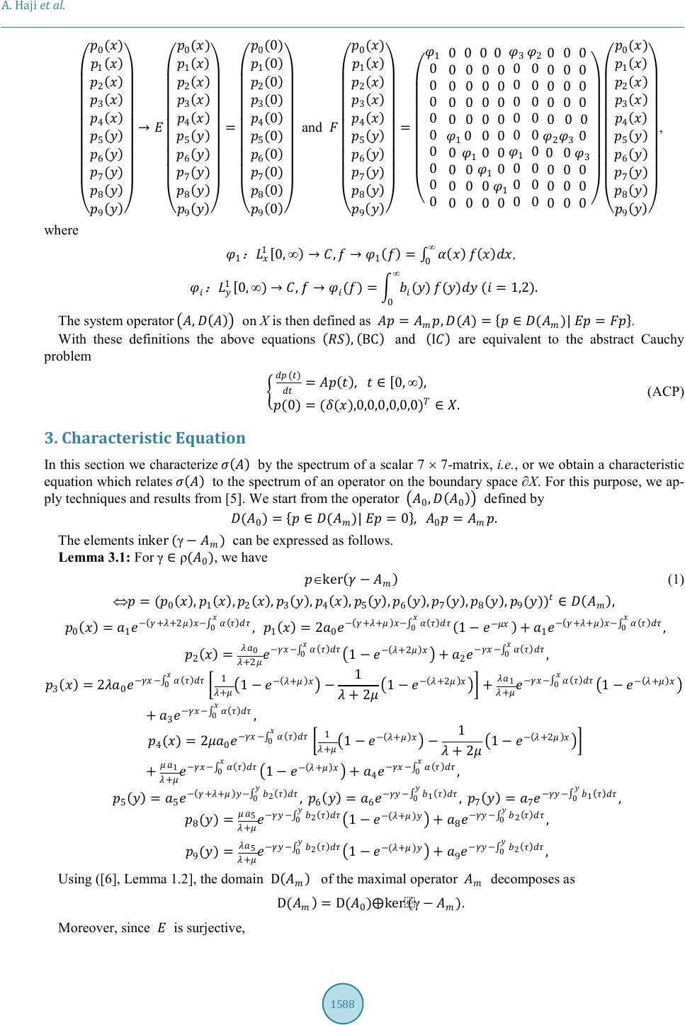 A. Haji et al. 0 ( ) 1 ( ) 2 ( ) 3 ( ) 4 ( ) 5 ( ) 6 ( ) 7 ( ) 8 ( ) 9 ( ) 0 ( ) 1 ( ) 2 ( ) 3 ( ) 4 ( ) 5 ( ) 6 ( ) 7 ( ) 8 ( ) 9 ( ) = 0 ( 0 ) 1 ( 0 ) 2 ( 0 ) 3 ( 0 ) 4 ( 0 ) 5 ( 0 ) 6 ( 0 ) 7 ( 0 ) 8 ( 0 ) 9 ( 0 ) and 0 ( ) 1 ( ) 2 ( ) 3 ( ) 4 ( ) 5 ( ) 6 ( ) 7 ( ) 8 ( ) 9 ( ) = 1 0 0 0 0 0 0 0 0 0 0 0 0 0 0 1 0 0 0 0 0 0 0 0 0 0 1 0 0 0 0 0 0 0 0 0 0 1 0 0 0 0 0 0 0 0 0 0 1 0 3 0 0 0 0 0 1 0 0 0 2 0 0 0 0 0 0 0 0 0 0 0 0 0 0 2 0 0 0 0 0 0 0 0 0 3 0 0 0 0 0 0 0 0 0 0 3 0 0 0 0 ( ) 1 ( ) 2 ( ) 3 ( ) 4 ( ) 5 ( ) 6 ( ) 7 ( ) 8 ( ) 9 ( ) , where 1 : 1 [ 0,∞ ) , 1 ( ) = ( ) ∞ 0 ( ) , : 1 [ 0,∞ ) , ( ) = ( ) ∞ 0 ( ) (=1,2). The system operator , ( ) on X is then defined as = , ( ) = { ( ) | = } . With these definitions the above equations ( ) , ( BC ) and ( I ) are equivalent to the abstract Cauchy problem () = ( ) , [ 0,∞ ) , ( 0 ) =((),0,0,0,0,0,0) . (ACP) 3. Characteristic Equation In this section we characterize ( ) by the spectrum of a scalar 7 × 7-matrix, i.e., or we obtain a characteristic equation which relates ( ) to the spectrum of an operator on the boundary space ∂X. For this purpose, we ap- ply techniques and results from [5]. We start from the operator 0 , ( 0 ) defined by ( 0 ) = { ( ) | =0 } , 0 = . The elements inker ( γ ) can be expressed as follows. Lemma 3.1: For γρ ( 0 ) , we have ∈ker ( ) (1) ⇔=( 0 ( ) , 1 ( ) , 2 ( ) , 3 ( ) , 4 ( ) , 5 ( ) , 6 ( ) , 7 ( ) , 8 ( ) , 9 ()) ( ) , 0 ( ) = 1 ( ++2 ) ( ) 0 , 1 ( ) =2 0 ( ++ ) ( ) 0 ( 1 ) + 1 ( ++ ) ( ) 0 , 2 ( ) = 0 +2 ( ) 0 1 ( +2 ) + 2 ( ) 0 , 3 ( ) =2 0 ( ) 0 1 + 1 ( + ) 1 + 2 1 ( +2 ) + 1 + ( ) 0 1 ( + ) + 3 ( ) 0 , 4 ( ) =2 0 ( ) 0 1 + 1 ( + ) 1 + 2 1 ( +2 ) + 1 + ( ) 0 1 ( + ) + 4 ( ) 0 , 5 ( ) = 5 ( ++ ) 2 ( ) 0 , 6 ( ) = 6 1 ( ) 0 , 7 ( ) = 7 1 ( ) 0 , 8 ( ) = 5 + 2 ( ) 0 1 (+) + 8 2 ( ) 0 , 9 ( ) = 5 + 2 ( ) 0 1 (+) + 9 2 ( ) 0 , Using ([6], Lemma 1.2], the domain D ( ) of the maximal operator decomposes as D ( ) =D( 0 )ker(γ ). Moreover, since is surjective, 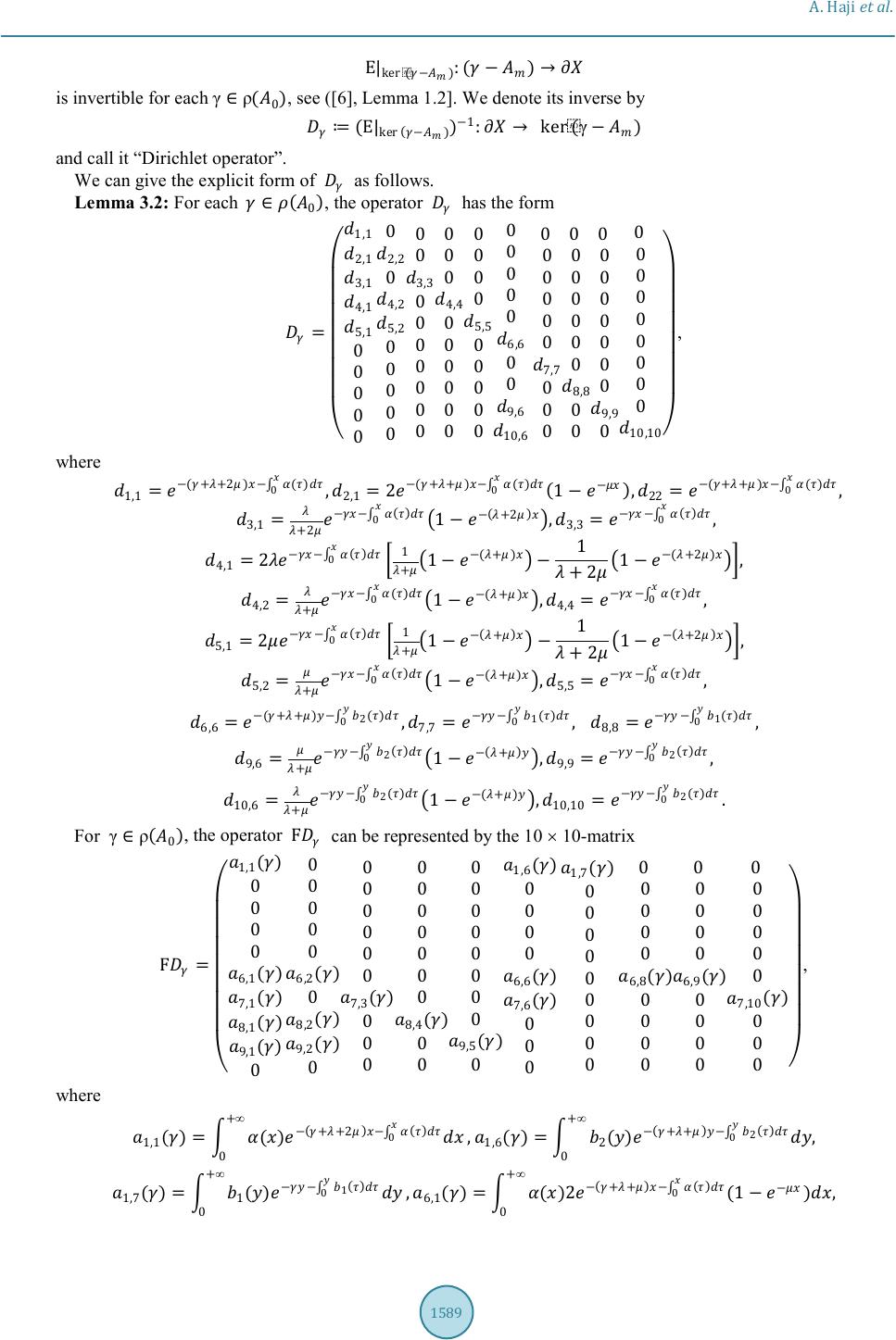 A. Haji et al. E| ker ( ) :( ) is invertible for each γρ ( 0 ) , see ([6], Lemma 1.2]. We denote its inverse by (E| ker ( ) ) 1 : ker(γ ) and call it “Dirichlet operator”. We can give the explicit form of as follows. Lemma 3.2: For each ( 0 ) , the operator has the form = 1,1 2,1 3,1 4,1 5,1 0 0 0 0 0 0 2,2 0 4,2 5,2 0 0 0 0 0 0 0 3,3 0 0 0 0 0 0 0 0 0 0 4,4 0 0 0 0 0 0 0 0 0 0 5,5 0 0 0 0 0 0 0 0 0 0 6,6 0 0 9,6 10,6 0 0 0 0 0 0 7,7 0 0 0 0 0 0 0 0 0 0 8,8 0 0 0 0 0 0 0 0 0 0 9,9 0 0 0 0 0 0 0 0 0 0 10,10 , where 1,1 = ( ++2 ) ( ) 0 , 2,1 =2 ( ++ ) ( ) 0 ( 1 ) , 22 = ( ++ ) ( ) 0 , 3,1 = +2 ( ) 0 1 ( +2 ) , 3,3 = ( ) 0 , 4,1 =2 ( ) 0 1 + 1 ( + ) 1 + 2 1 ( +2 ) , 4,2 = + ( ) 0 1 ( + ) , 4,4 = ( ) 0 , 5,1 =2 ( ) 0 1 + 1 ( + ) 1 + 2 1 ( +2 ) , 5,2 = + ( ) 0 1 (+) , 5,5 = ( ) 0 , 6,6 = ( ++ ) 2 ( ) 0 , 7,7 = 1 ( ) 0 , 8,8 = 1 ( ) 0 , 9,6 = + 2 ( ) 0 1 ( + ) , 9,9 = 2 ( ) 0 , 10,6 = + 2 ( ) 0 1 (+) , 10,10 = 2 ( ) 0 . For γρ ( 0 ) , the operator F can be represented by the 10 × 10-matrix F = 1,1 () 0 0 0 0 6,1 () 7,1 () 8,1 () 9,1 () 0 0 0 0 0 0 6,2 () 0 8,2 () 9,2 () 0 0 0 0 0 0 0 7,3 () 0 0 0 0 0 0 0 0 0 0 8,4 () 0 0 0 0 0 0 0 0 0 0 9,5 () 0 1,6 () 0 0 0 0 6,6 () 7,6 () 0 0 0 1,7 () 0 0 0 0 0 0 0 0 0 0 0 0 0 0 6,8 () 0 0 0 0 0 0 0 0 0 6,9 () 0 0 0 0 0 0 0 0 0 0 7,10 () 0 0 0 , where 1,1 ( ) = ( ) ( ++2 ) ( ) 0 +∞ 0 , 1,6 ( ) = 2 ( ) ( ++ ) 2 ( ) 0 +∞ 0 , 1,7 ( ) = 1 ( ) 1 ( ) 0 +∞ 0 , 6,1 ( ) = ( ) 2 ( ++ ) ( ) 0 ( 1 ) +∞ 0 ,  A. Haji et al. 6,2 ( ) = ( ) ( ++ ) ( ) 0 +∞ 0 , 6,6 ( ) = + 2 ( ) 2 ( ) 0 1 ( + ) , +∞ 0 7,1 ()= + 2 () ( ) 0 1 ( +2 ) +∞ 0 7,3 ( ) = ( ) +∞ 0 ( ) 0 , 7,6 ( ) = + 2 ( ) 2 ( ) 0 1 ( + ) +∞ 0 , 7,10 ( ) = 2 ( ) 2 ( ) 0 +∞ 0 , 8,1 ( ) = ( ) 2 ( ) 0 1 + 1 ( + ) 1 + 2 1 ( +2 ) , +∞ 0 8,2 ( ) = + ( ) ( ) 0 1 ( + ) , +∞ 0 8,4 ( ) = ( ) ( ) 0 +∞ 0 , 9,1 ()=()2 ( ) 0 [ 1 + 1 ( + ) 1 + 2 1 (+2) ], +∞ 0 9,2 ()= + () ( ) 0 1 (+) +∞ 0 , 9,5 ()=() ( ) 0 +∞ 0 . The Following result, which can be found in [7], plays important role for us to prove the existence of unique dynamic solution of the system. Lemma 3.3 (The characteristic equation): If ( 0 ) and there exists 0 such that 1 0 , then ( ) 1 . 4. Existence of a Unique Dynamic Solution of the System In this section, we prove the well-posedness and the existence of a unique positive dynamic solution of the sys- tem. For this purpose we first prove that the operator A generates a positive contraction 0 -semigroup ( ( ) ) 0 using the Phillips’ theorem, see ([8], Thm. C-II 1.2). The following lemma shows the surjectivity of for >0. Lemma 4.1: If, then ( ) . Proof: Let,>0. Then all the entries of are positive and using only elementary calculations one can show that the column sums are strictly less than 1. Hence, <1and thus 1 . Using Lemma 3.3 we conclude that ( ) . Lemma 4.2: (, ( ) )is a closed linear operator and ()is dense in. If ′ denotes the dual space of, then ′ =( ∞ ( [0,+∞ ) ) 5 × ( ∞ ( [0,+∞ ) ) 5 . It is obvious that ′ is a Banach space endowed with the norm =max( ∞ ( [0,+∞ ) , ∞ ( [0,+∞ ) ,=0,1,2,3,4,=5,6,7,8,9), where =( 0 ( ) , 1 ( ) , 2 ( ) , 3 ( ) , 4 ( ) , 5 ( ) , 6 (), 7 ( ) , 8 ( ) , 9 ()) ′ . Lemma 4.3: The operator , ( ) is dispersive. Proof: For p=( 0 ( ) , 1 ( ) , 2 ( ) , 3 ( ) , 4 ( ) , 5 ( ) , 6 ( ) , 7 ( ) , 8 ( ) , 9 ()) (), we define =( 0 ( ) , 1 ( ) , 2 ( ) , 3 ( ) , 4 ( ) , 5 ( ) , 6 (), 7 ( ) , 8 ( ) , 9 ()) ′ , where ( ) = | | + ( ) ,=0,1,2,3,4, ( ) = | | + ( ) ,=5,5,6,7,8,9 and + ( ) = 1 ( ) >0, 0 ( ) 0, =0,1,2,3,4, + ( ) = 1 ( ) >0, 0 ( ) 0, =5,6,7,8,9. Noting the boundary condition, it is not difficult to see that,0. By ([6], p. 49) we obtain that (, ( ) ) is a dispersive operator.  A. Haji et al. From Lemma 4.1-4.3 we see that all the conditions in Phillips’ theorem (see [8], Thm.C-II 1.2) are fulfilled and thus we obtain the following result. Theorem 4.4: The operator , ( ) generates a positive contraction 0 -semigroup ( ( ) ) 0 . From Theorem 4.4 and ([4], Cor.II.6.9) we can characterize the well-posedness of ()as follows. Theorem 4.5: The associated abstract Cauchy problem () is well-posed. From Theorem 4.5 and ([4], Prop. II.6.2) we can state our main result. Theorem 4.6: The system ( ) , ( ) and (I) has a unique positive dynamic solution p()=( 0 ( , ) , 1 ( , ) , 2 ( , ) , 3 ( , ) , 4 ( , ) , 5 ( , ) , 6 ( , ) , 7 ( , ) , 8 (,), 9 ( , ) . Acknowledgements This work was supported by the National Natural Science Foundation of Xinjiang Uighur Autonomous Region (No. 2014211A002). References [1] Li, W., Alfa, A.S. and Zhao, Y.Q. (l998) Stochastic Analysis of a Repairable System with Three Units and Two Repair Facilities. Microeletronics and Reliability, 38, 585-595. [2] Kovalenko, A.I. (2001) Analysis of the Reliability of a Three-Component System with Renewal. Journal of Mathe- matical Science, 103, 273-277. [3] Hu, L.M., Tian, R.L., Wu, J.B. and Cao, J. (2007) Reliability Analysis of Series-Parallel Repairable System Consisting of Three Units with Vacation. Journal of Y. Uni., 103, 299-303. [4] Engel, K.-J. and Nagel, R. (2000) One-Parameter Semigroups for Linear Evolution Equations. Graduate Texts in Ma- thematics, 194, Springer-Verlag. [5] Casarino, V., Engel, K.-J., Nagel, R. and Nickel, G. (2003) A Semigroup Approach to Boundary Feedback Systems. Integr. Equ. Oper. Theory, 47 , 289-306. http://dx.doi.org/10.1007/s00020-002-1163-2 [6] Greiner, G. (1987) Perturbing the Boundary Conditions of a Generator. Houston J. Math., 13, 213-229. [7] Haji, A. and Radl, A. (2007) A Semigroup Approach to Queueing Systems. Semigroup Forum, 75, 610-624. http://dx.doi.org/10.1007/s00233-007-0726-6 [8] Nagel, R. (1986) One-Parameter Semigroups of Positive Operators. Springer-Verlag. Submit or recommend next manuscript to SCIRP and we will provide best service for you: Accepting pre-submission inquiries through Email, Facebook, LinkedIn, Twitter, etc. A wide selection of journals (inclusive of 9 subjects, more than 200 journals) Providing 24-hour high-quality service User-friendly online submission system Fair and swift peer-review system Efficient typesetting and proofreading procedure Display of the result of downloads and visits, as well as the number of cited articles Maximum dissemination of your research work Submit your manuscript at: http://papersubmission.scirp.org/
|