J. Biomedical Science and Engineering, 2011, 4, 552-561
doi:10.4236/jbise.2011.48071 Published Online August 2011 (http://www.SciRP.org/journal/jbise/
JBiSE
).
Published Online August 2011 in SciRes. http://www.scirp.org/journal/JBiSE
Segmentation of MS lesions using entropy-based EM
algorithm and Markov random fields
Ahmad Bijar1, Mahdi Mohamad Khanloo1, Antonio Peñalver Benavent2, Rasoul Khayati1
1Department of Biomedical Engineering, Shahed University, Tehran, Iran;
2Department de Estadística, Matemáticas e Informática, Universidad Miguel Hernández, Elche, Spain.
Received 25 June 2011; revised 28 July 2011; accepted 8 August 2011.
ABSTRACT
This paper presents an approach for fully automatic
segmentation of MS lesions in fluid attenuated inver-
sion recovery (FLAIR) Magnetic Resonance (MR)
images. The proposed method estimates a gaussian
mixture model with three kernels as cerebrospinal
fluid (CSF), normal tissue and Multiple Sclerosis le-
sions. To estimate this model, an automatic Entropy
based EM a lgo r it h m is u s ed to f ind th e b est es t ima ted
Model. Then, Markov random field (MRF) model
and EM algorithm are utilized to obtain and upgrade
the class conditional pro bability density function and
the apriori probability of each class. After estimation
of Model parameters and apriori probability, brain
tissues are classified using bayesian classification. To
evaluate the result of the proposed method, similarity
criteria of different slices related to 20 MS patients
are calculated and compared with other methods
which include manual segmentation. Also, volume of
segmented lesions are computed and compared with
gold standard using correlation coefficient. The pro-
posed method has better performance in comparison
with previous works which are reported here.
Keywords: Gaussian Mixture Model; EM; Entropy;
Markov Random Field; Multiple Sclerosis
1. INTRODUCTION
Magnetic Resonance Imaging (MRI) permits the non-
invasive detailed visualization of internal anatomical
structures. The segmentation of MR images into ana-
tomical tissues, fluids, and structures is an area of inter-
est in MRI, and is increasingly being used to assess the
progression of the disease and to evaluate the effect of
drug therapy, supplementing traditional neurological
disability scales such as the extended disability status
scale (EDSS) [1]. Multiple Sclerosis (MS) is a chronic,
inflammatory, demyelinating disease of the Central
Nervous System (CNS) that primarily affects the white
matter (WM) of the central nervous system. MS lesions
exhibit hypersignals in T2 weighted and hyposignals in
T1 weighted, with respect to normal white matter inten-
sities. Previous research has shown that the FLAIR
(Fluid Attenuated Inversion Recovery) sequence con-
tains the most distinctive lesion-healthy tissue differen-
tiation for segmentation of white matter lesions. The
radiological criteria for MS include the number of lesion
on the MRI, their locations and their sizes, and these
quantitative information is also crucial for studying the
progression of MS lesions and the effect of drug treat-
ments. To make a quantitative analysis of the brain scans
of the patient, human experts are required to identify the
multiple sclerosis lesions that are present in those scans
as manual segmentation which is extremely time con-
suming. So, automatic and semi-automatic methods for
segmentation of MS lesions are recommended and have
been investigated extensively. There are many proposed
approaches, automatic and semi-automatic, for segmen-
tation of brain into different tissues, including MS le-
sions. These approaches include a variety of methods
such as statistical, fuzzy, neural networks, and fuzzy
neural networks. In this paper, we develop a fully auto-
matic method for segmentation of MS lesions that re-
quires no training, atlas, or thresholding steps. Our
method can be divided into two main sections: at first,
intensities of brain pixels are modeled using a gaussian
mixture model which consists of three kernels as CSF,
normal tissue and MS lesions classes. This step starts
with only one kernel and uses an entropy based EM al-
gorithm to estimate three kernels as three mentioned
classes in an automatic manner which does not need
initial values for parameter estimation. After estimation
of the model, we would be able to classify brain pixels
by knowing apriori probabilities of the classes. The next
step is obtaining these apriori probabilities with no
training and atlas. So, a MRF model and EM algorithm

A. Bijar et al. / J. Biomedical Science and Engineering 4 (2011) 552-561 553
are applied to update and attain apriori probabilities and
means and variances of each class.
2. METHODS
2.1. Patients and MR Imaging
The proposed method is evaluated on a dataset which is
obtained and used in [2]. This dataset contains 16 female
and 4 male with average age of 29 ± 8 years old, this
dataset is selected according to the revised Mc Donald
criteria 2005 [3]. All images were acquired according to
full field MRI criteria of MS [3] in T2-weighted (T2-w),
T1-weighted (T1-w), Gadolinium enhanced T1-weighted,
and FLAIR in axial, sagittal and coronal surfaces. We
selected the FLAIR images, especially axial ones, with
lesions in deep, priventricular, subcortical, and cortical
white matters (supratentorial lesions). More lesion load
and higher accuracy of FLAIR in revealing of these MS
lesions were the reason for this selection [4]. Each image
volume (patient data) consisted of averagely 40 slices
with a 256 × 256 scan matrix. The pixel size was 1mm2,
and the slice thickness was 3mm without any gap.
2.2. Manual Segmentation of MS Lesions and
Brain Segmentation
The segmentation of MS lesions was performed manu-
ally by neurologist and radiologist in Flair images with
visual inspection of corresponding T1-w and T2-w im-
ages. These manually segmented images were used as
Gold standard [5] to evaluate the performance of pro-
posed method. To evaluate the proposed method, differ-
ent types of images which have different lesion volumes
were applied. Also, the brain segmentation was per-
formed using a fully automatic object-oriented approach
[6]. This method was based on the regional-spatial char-
acteristics of brain in MR images. At first, original im-
age is converted to a binary image. Then, morphological
opening on the binary image is performed and tiny re-
gions are eliminated. Three rectangular masks showing
the cerebral regions are produced and the regions in the
binary image which have overlap with these rectangles
are preserved and, the rest are eliminated. Final mask is
generated by dilation of selected regions and filling tiny
holes. Finally, an image, which includes only cerebral
tissues, is obtained by applying the resulted mask on the
original image.
3. PROBLEM FORMULATION
3.1. Gaussian Mixture Model
A finite mixture model is the weighted sum of M
> 1 components in for

xp
n
n
1
 
1
xπxx
Mn
m
m
ppm



M
(1)
where corresponds to the
weight of each component which satisfies
 
π0,11,2,,
mm
1mπ1
M
m

.
For the Gaussian mixtures model, each component den-
sity


xpm is a Gaussian probability density given by




xm 
1
2 2
1
x
2πdet
1
exp x
2
mn
m
T
mm
p  
 (2)


 



where T denotes the transpose operation, m

is the
mean vector and m

is the covariance matrix which is
assumed positive definite. Here we encapsulate these
parameters into a parameter vector, writing the parame-
ters of each component asmmm
to get

 

,,


12
π,π,,π, ,.  
12
,,
m

m
Eq.1 can be rewritten as

 
1
xπx

mm
m
pp
M


 (3)

If we knew the component from which x came, then it
would be simple to determine the parameters

. Simi-
larly, if we knew the parameters , we could determine
the component that would be most likely to have pro-
duced x. The difficulty is that we know neither.

3.2. Bayesian Classification
Bayesian Classification is a probabilistic technique of
pattern recognition and is based on the principle of
Bayes decision theory [7], given in Eq.4 below





j
j
j
px P
Px px




 (4)
where, x is a given feature vector,
j

denotes a class,
or state of nature,


j
P

is the prior probability of
class
j

,


px is prior probability of the feature vec-
tor x,


j
px

is aposteriori probability, which a fea-
ture vector should be classified as belonging to class
j

,


j
P
x 
is the conditional probability that a feature
vector occurs in a given class
j

. For the approach here,
the feature x shall consist of one component, intensity of
brain pixels. The quantity is known as the evi-
dence, and serves only as a scale factor, such that the
quantity in Eq.4 is indeed a true probability, with values
between zero and one. So, the maximum a posteriori
(MAP) estimate of Eq.4 is used as below

px



 
j
jj
Pxpx P

  (5)
According to Bayesian theory [8], the feature vector x
is classified to
j

of which the aposteriori probability
given x is the largest between the classes.






max
jj
iii
px P
px P

j
x

 

 (6)
C
opyright © 2011 SciRes. JBiSE

A. Bijar et al. / J. Biomedical Science and Engineering 4 (2011) 552-561 554
Bayes decision rule is optimal in the sense of minimi-
zation of the probability of error. It is quite obvious that
such an Ideal Bayesian solution can be used only if dis-
tributions

j
px

, and the apriori probabilitles


j
P

are known. In the context of classification of brain tissue,
the probability models are not known, and therefore,
must be approximated. The performance of the Bayesian
classifier is directly related to how well these distribu-
tions can be modeled.
3.3. EM Algorithm
The Expectation-Maximization (EM) algorithm [9] is a
general-purpose iterative algorithm for maximum likeli-
hood (ML) estimation.The EM algorithm consists of two
steps, E-step (expectation) and M-step (maximization)
which are alternately used until the


1
log n
i
ipx 


converges to a local optimum. Let

,1,,
i
X
xi n
be a set of n realizations of a random d-dimensional
vector χ with a pdf . Thus the parameterized pdf
can be written as a combination of pdfs of the M com-
ponents m characterizing the finite
mixture model

i
px
,M

1,wm

 
1π
M
im
m
px px

im



 (7)
The likelihood can be expressed as
  
1 11
π
nn M
im
m
ii
Lpx px

im

 
 
 (8)
E-step: the data χ are assumed to be incomplete and
the complete data set is determined by es-
timating the set of variables

,Y  

Z

12
,, M
Z
ZZ Z, where
each
M
Z
is an N-dimensional vector .
The log likelihood of the complete data Y is
T
,
N
m
z


12
,,
mm
zz
 
11
loglog πx
NM
ii
mm m
im
pYz p 
 
 
 (9)
where
 


1
πx
x,
πx
tit
mm
iit
mMtit
ll
l
p
zPm
p




 (10)
is the posterior probability and is the parameter
estimate obtained after t iterations.
t

M-step: in this step, the parameters are deter-
mined according to the estimate of the variables . For
Gaussian mixture models this corresponds to reestimat-
ing the , the
1t

i
m
z
1
πt
m
1t
m

 and 1t
m


for each m according
to:
1
1
1
πN
t
m
iz
N


i
m
(11)
11
1
x
Ni
mi
ti
mNi
m
i
z
z




 (12)

111
11
1
xx
T
tit t
mi mi m
ti
N mi
m
i
z
z






 (13)
4. ENTROPY
In the information theory, information entropy is a
measurement of the system uncertain degree. The term
of entropy in the theory of information was first intro-
duced by Shannon, in 1948, in [10].
4.1. Shannon Entropy
Let


1,, n
X
xx be a discrete random variable with
values in S and probability mass function


px, the
information (or uncertainty) of each possible event is


log
i

i
I
xp x (14)
The mean of


I
X is introduced as Shannon en-
tropy and is denoted by


H
X





 


log
xs
H
XEI Xpxpx


 (15)


H
X varies from zero to

log S zero meaning that
there is no uncertainty, whereas

log S is reached
when all elements of X have equal probabilities, in this
case, the uncertainty is at its maximum [11].
4.2. Rényi Entropy
Rényi further expanded the concept of Sannon entropy,
and defined the


0, 1qq q order Rényi [12] en-
tropy of probability density function as

px
 
1log, 1
1
q
qxs
HXpx q
q


 (16)
Rényi entropy is a non-increasing function of q and It
can be verified, by applying the 1’Hôpital rule that
Shannons entropy is the Rényi entropy of order 1.
5. ENTROPY ESTIMATION
In this paper, Rényi entropy [12] is selected as entropy
measure and estimation of this type of entropy which
will be express, is based on Leonenko and et al. [13].
Let n
X

 be a random vector with probability
measure μ having the density p. The proposed method
by Leonenko estimates q
H
from a sample of N inde-
pendent and identically distributed (i.i.d.) random vari-
ables 12 N based on the nearest neigh-
bor distances in the sample. This work is resumption of
the method which estimates
,,XX,X N 2
1
H
and proposed by Ko-
zachenko and Leonenko [14].
Leonenko’s method estimates q, Eq.17, for I1q

through the computation of conditional moments of
nearest-neighbor distances.
 



1,
q
q
qq xs
IIppxpx q

1



 (17)
C
opyright © 2011 SciRes. JBiSE

A. Bijar et al. / J. Biomedical Science and Engineering 4 (2011) 552-561 555
5.1. Estimators
Suppose that 12 , are i.i.d. with a
probability measure μ having a density p with respect to
the Lebesgue measure. Let
,,, 2
N
XXX N


,
x
y  denote the Euclid-
ean distance between two points ,
x
y of . For a
given sample
m

1,
N
X
X and a given i
X
in the sample,
from the distances 1N

ij
,, 1,,,
X
Xj N

i





the order statistics 1, 12, 11, 1
NN
,ji

ii
NN


are formed, so that is the kth nearest-neighbor
distance from i


,1
i
kN


X
to some other
j
X
in the sample,
.jiq
I
in Eq.18 is estimated for , by 1q

1
,, ,,
1
ˆq
Nkq Nik
IN

ζ (18)
where



,,, 1
1
m
i
Nikk mkN
NCV 

ζ


2
π21
m
m
Vm
( is the volume of the unit ball in )
m
V

0, 1 
m

 

11q
1
k
Ckkq  

So, q
H
in Eq.17 is estimated as below



,, ,,
ˆ
log 1
NKq Nkq
H
Iq (19)
5.2. Maximum Entropy
Suppose that we have a group of variables which have
obtained from different types of distributions and have
equal variance. According to the second Gibbs theorem
[15], among all of them, Gaussian variables have maxi-
mum entropy. Therefor, by using this theorem, we
would be able to understand that if the modeling of the
variable with a gaussian kernel is acceptable or not. This
procedure is done through the comparing of the theo-
retical maximum entropy and the real one of the under-
lying data. Let X be a d dimensional variable, the theo-
retical maximum entropy is computed as below
 
max
1log 2π
2
d
HX  



(20)
where, is covariance of observations. There would
be no difference between the theoretical maximum en-
tropy and the real one. If the data were truly Gaussian.
We have used this property to determine the worst esti-
mated kernel in the mixture.

6. SELECTION AND SPLIT OF THE
WORST ESTIMATED KERNEL
For every kernel in the mixture, the theoretical maxi-
mum entropy and the real one of the underlying data is
computed and evaluated in the normalized weighted
form [16] to find the worst estimated kernel. The worst
estimated kernel would be selected through
 

max real
max
arg maxπ
kk
H
kH k
kHk


 








(21)
where, k

indicates the worst estimated kernel,


real
H
k is the real entropy of the data under the kth
kernel, and


max
H
k is the maximum entropy of the
kth kernel. Suppose that a special kernel has been se-
lected to split, during the split step, overall dispersion
and two new covariance matrices have to be constant
and positive define, respectively. If the kth component
had to split into the k1th and k2th components, the first
two moments, the mean vectors and the covariance ma-
trices should satisfy the following split equations which
are proposed by Richardson and Green [17]
12
112 2
πππ
ππ π
kkk
kkkkkk
 






11112 222
π
ππ
T
kk kk
TT
kkkkk kkk





 
(22)
Solving the split equations is an ill-posed problem
because the number of the equations is less than the
number of the unknowns. To solve this ill-posed prob-
lem, we have used the method which is proposed by
Dellaportas and Papageorgiou in [18]. They have used
the spectral decomposition of the current covariance
matrix, and the original problem is replaced by estimat-
ing the new eigenvalues and eigenvectors of the new
covariance matrices without the previously cited con-
straint. Let k the spectral decomposition
of the covariance matrix
VV
T
kkk
 
k

, with , the eigenvector
matrix,
Vk


1
diag ,d
kkk

   a diagonal matrix con-
taining the eigenvalues of k
 with increasing order,
and d the problem dimension. Let also D be a d × d rota-
tion matrix with orthonormal unit vectors as columns. D
is built by generating its lower triangular matrix inde-
pendently from


12dd different uniform U(0,1)
densities. The proposed split operation is given by



 
 
11
21
2
1
1
1
2
2
1
2
2
1
2
1
322
322
ππ
π1π
π
Vπ
π
Vπ
diag diagdiag
diagdiagdiag 1
kkk
kkk
dk
iii
kk kk
i
k
dk
iii
kk kk
i
k
kk
kk
u
u
uuu
uuu


 
 










 



C
opyright © 2011 SciRes. JBiSE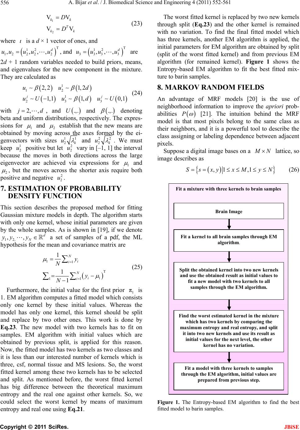

A. Bijar et al. / J. Biomedical Science and Engineering 4 (2011) 552-561 556
1
2
VV
VV
k
T
kk
D
D


k
(23)
where

is a d × 1 vector of ones, and

T
12
12 222
,,,,
d
uuu uu, and are

T
12
333 3
,,,
d
uuu u
2d + 1 random variables needed to build priors, means,
and eigenvalues for the new component in the mixture.
They are calculated as



 
1
12
1
233
2, 21,2
1,1 1,0,1
j
uud
uUu duU

 



j
d
(24)
with , and and denoting
beta and uniform distributions, respectively. The expres-
sions for 1
2, ,j

.,.U

.,. 

and 2

establish that the new means are
obtained by moving across the axes formed by the ei-
genvectors with sizes 11
2k
u

and 22
2k
u

. We must
keep positive but let vary in [–1, 1] the interval
because the moves in both directions across the large
eigenvector are achieved via expressions for 1
1
2
u2
2
u

and
2

, but the moves across the shorter axis require both
positive and negative .
2
2
u
7. ESTIMATION OF PROBABILITY
DENSITY FUNCTION
This section describes the proposed method for fitting
Gaussian mixture models in depth. The algorithm starts
with only one kernel, whose initial parameters are given
by the whole samples. As is shown in [19], if we denote
12, a set of samples of a pdf, the ML
hypothesis for the mean and covariance matrix are
,, d
N
yy y

11
T
1
11
1
1
1
N
i
i
N
i
i
y
N
y
N









(25)
Furthermore, the initial value for the first prior 1 is
1. EM algorithm computes a fitted model which consists
only one kernel by these initial values. Whereas the
model has only one kernel, this kernel should be split
and replace by two other ones. This work is done by
Eq.23. The new model with two kernels has to fit on
samples. EM algorithm with initial values which are
obtained by previous split, is applied for this reason.
Now, the fitted model has two kernels as two classes and
it is less than our interested number of kernels which is
three, csf, normal tissue and MS lesions. So, the worst
fitted kernel among these two kernels has to be selected
and split. As mentioned before, the worst fitted kernel
has big difference between the theoretical maximum
entropy and the real one against other kernels. So, we
could select the worst kernel by means of maximum
entropy and real one using Eq.21.
π
The worst fitted kernel is replaced by two new kernels
through split (Eq.23) and the other kernel is remained
with no variation. To find the final fitted model which
has three kernels, another EM algorithm is applied, the
initial parameters for EM algorithm are obtained by split
(split of the worst fitted kernel) and from previous EM
algorithm (for remained kernel). Figure 1 shows the
Entropy-based EM algorithm to fit the best fitted mix-
ture to barin samples.
8. MARKOV RANDOM FIELDS
An advantage of MRF models [20] is the use of
neighborhood information to improve the apriori prob-
abilities


P

[21]. The intuition behind the MRF
model is that most pixels belong to the same class as
their neighbors, and it is a powerful tool to describe the
class assigning or labeling dependence between adjacent
pixels.
Suppose a digital image bases on a
M
N lattice, so
image describes as




,1 ,1SsxyxM yN (26)
Fit a mixture with three kernels to brain samples

Brain Image
Fit a kernel to all brain samples through EM
algorithm.
Split the obtained kernel into two new kernels
and use the obtained result as initial values to
fit a new model with two kernels to all
samples through the EM algorithm.
Find the worst estimated kernel in the mixture
which has two kernels by comparing the
maximum entropy and real entropy, and split
it into two new kernels and use its result as
initial values for the next level , the other
kernel has no variation .
Fit a model w ith three kernels to samples
through the EM algorithm, initial values are
prepared from previous step.
Figure 1. The Entropy-based EM algorithm to find the best
fitted model to barin samples.
C
opyright © 2011 SciRes. JBiSE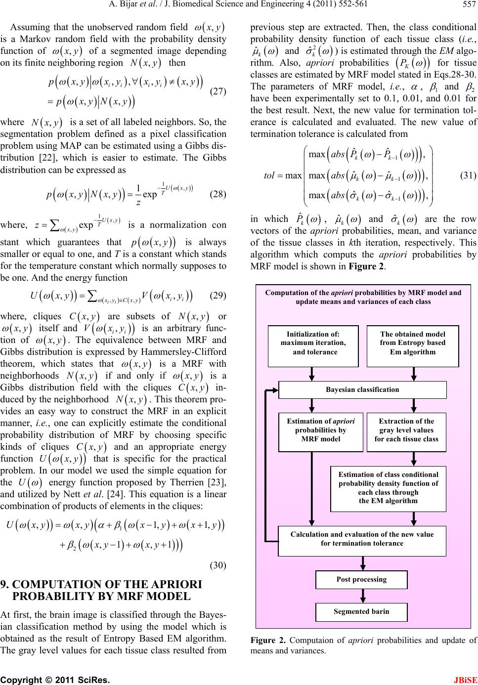

A. Bijar et al. / J. Biomedical Science and Engineering 4 (2011) 552-561 557
Assuming that the unobserved random field


,
x
y 
is a Markov random field with the probability density
function of

,

x
y  of a segmented image depending
on its finite neighboring region then

,Nxy







,,,,,
,,
ii ii
pxy xyxyxy
pxyNxy





(27)
where is a set of all labeled neighbors. So, the
segmentation problem defined as a pixel classification
problem using MAP can be estimated using a Gibbs dis-
tribution [22], which is easier to estimate. The Gibbs
distribution can be expressed as

,Nxy


 
1,
1
,,exp
Uxy
T
pxyNxy z





(28)
where,


1,
,exp Uxy
T
xy
z


 is a normalization con
stant which guarantees that is always
smaller or equal to one, and T is a constant which stands
for the temperature constant which normally supposes to
be one. And the energy function
 
,pxy 

 
 



,,
,,
ii ii
xy Cxy
Uxy Vxy



 (29)
where, cliques are subsets of or

,Cxy
 

,Nxy

,
x
y  itself and



,
ii
Vxy 

is an arbitrary func-
tion of

,
x
y  . The equivalence between MRF and
Gibbs distribution is expressed by Hammersley-Clifford
theorem, which states that

,

x
y  is a MRF with
neighborhoods if and only if

,Nxy

,
x
y 

,Cxy
is a
Gibbs distribution field with the cliques in-
duced by the neighborhood


y,Nx

. This theorem pro-
vides an easy way to construct the MRF in an explicit
manner, i.e., one can explicitly estimate the conditional
probability distribution of MRF by choosing specific
kinds of cliques and an appropriate energy
function that is specific for the practical
problem. In our model we used the simple equation for
the

,Cxy


,yUx 

U

energy function proposed by Therrien [23],
and utilized by Nett et al. [24]. This equation is a linear
combination of products of elements in the cliques:
   




 
1
2
, ,1,1,
,1 ,1
Uxyxyxy xy
xy xy
 
 


(30)
9. COMPUTATION OF THE APRIORI
PROBABILITY BY MRF MODEL
At first, the brain image is classified through the Bayes-
ian classification method by using the model which is
obtained as the result of Entropy Based EM algorithm.
The gray level values for each tissue class resulted from
previous step are extracted. Then, the class conditional
probability density function of each tissue class (i.e.,


ˆk

 and


2
ˆk

 ) is estimated through the EM algo-
rithm. Also, apriori probabilities
 
K
P


for tissue
classes are estimated by MRF model stated in Eqs.28-30.
The parameters of MRF model, i.e.,

, 1

and 2

have been experimentally set to 0.1, 0.01, and 0.01 for
the best result. Next, the new value for termination tol-
erance is calculated and evaluated. The new value of
termination tolerance is calculated from
 




 


 

1
1
1
ˆˆ
max ,
ˆˆ max max,
ˆˆ
max ,
kk
kk
kk
abs PP
tol abs
abs

 
 













(31)
in which


ˆk
P

,


ˆk

 and

ˆk

 are the row
vectors of the apriori probabilities, mean, and variance
of the tissue classes in kth iteration, respectively. This
algorithm which computs the apriori probabilities by
MRF model is shown in Figure 2.
Computation of the apriori probabilities by MRF model and
update means and variances of each class
The obtained model
from Entropy based
Em algorithm
Initialization of:
maximum iteration,
and tolerance
Bayesian classification
Extraction of the
gray level values
for each tissue class
Estimation of apriori
probabili ties by
MRF model
Estimation of class conditional
probabili ty density function of
each class through
the EM algorithm
Calculation and evaluation of the new value
for termination tolerance
Post processing
Segmented barin
Figure 2. Computaion of apriori probabilities and update of
means and variances.
C
opyright © 2011 SciRes. JBiSE

A. Bijar et al. / J. Biomedical Science and Engineering 4 (2011) 552-561 558
10. POSTPROCESSING
In manual segmentation, the possible lesions with sizes
as small as one or two pixels are not usually considered
as MS lesions by experts. However, as the gray level of
neighboring pixels in an image usually are highly corre-
lated, in our approach, the one-pixel object is considered
as a possible noise if its gray level is higher than the
average gray levels of its neighbor pixels (in 3 × 3
neighborhood) plus a margin of 25 (which is selected by
trial). This object is recognized as noise and removed in
the next step. Regarding the two pixel objects, in con-
trast with the manual procedure, these objects may be
identified as seed points of MS lesions as recommended
by the neurologist.
JBiSE
11. SIMULATION RESULTS
The results of proposed method, for two slices which
contain different lesion loads are shown in Figure 3 and
Figure 4. Segmented brain of typical original FLAIR
images are shown in Figure 3(a) and Figure 4(a). Mul-
tiple sclerosis pixels and the resulting segmented slices
are shown in Figure 3(b) and Figure 4(b). Figure 3(c)
and Figure 4(c) show the histogram of brain pixels and
estimated distribution through the proposed method.
Also, three estimated kernels which constitute gaussian
mixture model are shown in Figure 3(d) and Figure
4(d).
12. EVALUATION
To evaluate the proposed method, SI [25], OF and EF
[26] criteria are considered and computed over all 20
patients.
2TP
SI 2TPFPFN

 (32)
Figure 3. Result of applying the proposed algorithm to the image of a patient: (a) brain image; (b) result of
proposed method; (c) histogram of brain, overlaid.

A. Bijar et al. / J. Biomedical Science and Engineering 4 (2011) 552-561 559
Figure 4. Result of applying the proposed algorithm to the image of a patient: (a) brain image; (b) result of proposed method; (c)
histogram of brain, overlaid.
TP
OF TP FN  (33)
FP
EF TP FN  (34)
where, TP stands for true positive voxels, FP for false
positive voxels, and FN for false negative voxels. SI and
OF for a good segmentation should be close to 1 and EF
should be close to 0. As mentioned before, patients are
categorized into 3 groups. The proposed method has
been applied to all patients and SI, OF and EF criteria
are computed and mean values of each group are illus-
trated in Table 1. It is noticeable that SI, OF and EF are
improved with an increase in lesion load. Also, the
volumetric comparison of lesions between the proposed
method and gold standard using correlation coefficient
(CC) for each patient group is shown in Table 1. By
attention to correlation coefficient values, accuracy of
the proposed method is increased for patients with large
lesion load.
13. CONCLUSIONS
In this paper, we have described and validated a fully
automatic method for classification of brain tissues in
MR FLAIR images of MS patients. A gaussian mixture
model which has three kernels as brain tissues is ob-
tained through entropy based EM algorithm. This task
starts with only one kernel and finally finds three kernels
with no initially supplied training samples. Then, apriori
probabilities of classes are estimated using MRF. At last,
brain tissues are classified through Bayesian Classifica-
tion. This framework has been validated on a data set of
C
opyright © 2011 SciRes. JBiSE

A. Bijar et al. / J. Biomedical Science and Engineering 4 (2011) 552-561 560
Table 1. Similarity criteria and volumetric comparison of lesions for each patient group.
Correlation analysis Similarity criteria
Correlation CoefficientM ± SD (CC) MGS ± SDGS (CC) EF OF SI
N Patient category
0.93 1.87 ± 1.11 1.89 ± 1.13 0.27230.7277 0.7262 7 Small lesion load
0.95 11.58 ± 3.08 11.59 ± 3.10 0.22010.7395 0.7531 10 Moderate lesion load
0.98 22.23 ± 3.52 22.21 ± 3.54 0.15410.7857 0.8101 3 Large lesion load
N: number of patients in each group, M: mean, SD: standard deviation
Table 2. Similarity index (SI) values for the proposed method
and the other methods.
Method Similarity index (SI)
Johnston et al. [3] 0.65
Boudraa et al. [13] 0.62
Leemput et al. [14] 0.51
Zijdenbos et al. [31] 0.68
Proposed Method 0.75
MR FLAIR images of 20 MS patients via similarity cri-
teria (i.e., SI, OF, and EF). There are other segmentation
methods which have been evaluated via similar ways
(i.e., SI), and have used manual segmentation for
evaluation of them, such as Johnston et al. [27], Boudraa
et al. [28], Leemput et al. [29], and Zijdenbos et al. [30].
Comparison of proposed method with these methods is
shown in Table 2. Johnston et al. [31] presented a semi-
automatic segmentation approach based on stochastic
relaxation method (SRM) and iterated conditional mode.
Boudraa et al. [28] performed an automatic detection of
MS lesions by using fuzzy C-means (FCM) algorithm.
Leemput et al. [29] proposed the use of an intensity-
based and stochastic model-aided segmentation ap-
proach for fully automatic segmentation of MS lesions.
Zijdenbos et al. [30] developed an automatic pipeline
based on a supervised artificial neural network (ANN)
classifier. As it is seen in Table 2, the proposed method
has improved the results reported in [26-29]. Also, in
[31], it is mentioned that a value for SI more than 0.7
represents a very good segmentation in this field. Future
work will include improving accuracy and correlation
value.
REFERENCES
[1] Kurtzke, J.F. (1983) Rating neurologic impairment in
multiple sclerosis: An expanded disability status scale
(EDSS). Neurology, 33, 1444-1452.
[2] Rasoul, K., Mansur, V., Farzad, T., Massood Nabavi., S.
(2008) Fully automatic segmentation of multiple sclero-
sis lesions in brain MR FLAIR images using adaptive
mixtures method and Markov random field model. Com-
puters in Biology and Medicine, 38, 379-390.
doi:10.1016/j.compbiomed.2007.12.005
[3] Polman, C.H., Reingold, S.C., Edan, G., Fillippi, M.,
Hartung, HP. and Kappos, L. (2005) Diagnostic criteria
for MS 2005 revisions to the MC Donald criteria. Annals
of Neurology, 58, 840-846. doi:10.1002/ana.20703
[4] Edelman, R.R., Hesselink, J.R. and Zlatkin, M.B. (2006)
Clinical magnetic resonance imaging. 3rd Edition, Saun-
ders, Philadelphia, 1571-1615.
[5] Anbeek, P., Vincken, K.L., van Osch, M.J.P., Bisschops,
R.H.C. and Van der Grond, J. (2004) Probabilistic seg-
mentation of white matter lesions in MR imaging,
NeuroImage, 21, 1037-1044.
doi:10.1016/j.neuroimage.2003.10.012
[6] Khayati, R. (2006) Quantification of multiple sclerosis
lesions based on fractal analysis. PhD Thesis, Technical
Report No. 1: Fully automatic object oriented brain seg-
mentation in MRI. Amirkabir University of Technology,
Tehran.
[7] Duda, R.O., Hart, P.E. and Stork, D.G. (2001) Pattern
classification. 2nd Edition, Wiley, New York.
[8] Bernardo, J.M. and Smith, A.F.M. (1994) Bayesian the-
ory. Wiley, New York. doi:10.1002/9780470316870
[9] Dempster, A.P., Laird, N.M. and Rubin, D.B. (1997)
Maximun likelihood from incomplete data via the EM
algorithm. Journal of the Royal Statistical Soceity B, 39,
1-38. doi:10.1.1.133.4884
[10] Shannon, C. (1948) A mathematical theory of communi-
cation. Bell System Technical Journal, 27, 379-423.
[11] Cover, T.M. and Thomas, J.A. (1991) Elements of infor-
mation theory. Wiley & Sons, New York.
doi:10.1002/0471200611
[12] Renyi, A. (1961) On measures of entropy and informa-
tion. University California Press, Berkeley, 547-561.
[13] Leonenko, N., Pronzato, L. and Savani, V. (2008) A class
of Rényi information estimators for multidimensional
densities. Annals of Statistics, 36, 2153-2182.
doi:10.1214/07-AOS539
[14] Kozachenko, L. and Leonenko, N. (1987) On statistical
estimation of entropy of a random vector. Problems In-
formation Transmission, 23, 95101.
[15] Jones, M. and Sibson, R. (1987) What is projection pur-
suit. Journal of the Royal Statistical Society: Series A,
150, 136. http://www.jstor.org/stable/2981662
[16] Benavent, A.P. Ruiz, F.E. and Sáez, J.M. (2009) Learning
Gaussian mixture models with entropy-based criteria.
IEEE Transactions on Neural Networks, 20, 1756-1771.
doi:10.1109/TNN.2009.2030190
[17] Richardson, S. and Green, P. (1991) On Bayesian analy-
sis of mixtures with an unknown number of components
(with discussion). Journal of the Royal Statistical Society:
C
opyright © 2011 SciRes. JBiSE

A. Bijar et al. / J. Biomedical Science and Engineering 4 (2011) 552-561 561
Series B, 59, 731-792. doi:10.1111/1467-9868.00095
[18] Dellaportas, P. and Papageorgiou, I. (2006) Multivariate
mixtures of normals with unknown number of compo-
nents. Statistics and Computing, 16, 57-68.
doi:10.1007/s11222-006-5338-6
[19] Mitchell, T.M. (1997) Machine Learning. McGraw-Hill,
Boston. doi:10.1036/0070428077
[20] Li, S.Z. (2001) Markov random field modeling in image
analysis. Springer, Tokyo.
[21] Held, K., Kops, E.R., Krause, B.J., Wells, W.M., Kikinis,
R. and Mller-Grtner, H.W. (1997) Markov random field
segmentation of brain MR images. IEEE Transactions on
Medical Imaging, 16, 878-886. doi:10.1109/42.650883
[22] Geman, D., Geman, S., Graffigne, C. and Dong, P. (1990)
Boundary detection by constrained optimization, IEEE
Transactions on Pattern Analysis and Machine Intelli-
gence, PAMI-12, 609-628. doi:10.1109/34.56204
[23] Therrien, C.W. (1989) Decision, estimation, and classifi-
cation. Wiley, New York.
[24] Nett, J.M. (2001) The study of MS using MRI, image
processing, and visualization. Master’s Thesis, Univer-
sity of Louisville, Louisville.
[25] Zijdenbos, A.P., Dawant, B.M., Margolin, R.A. and Palmer,
A.C. (1994) Morphometric analysis of white matter lesions
in MR images: Method and validation. IEEE Transactions
on Medical Imaging, 13, 716-724.
doi:10.1109/42.363096
[26] Stokking, R., Vincken, K.L. and Viergever, M.A. (2000)
Automatic morphologybased brain segmentation
(MBRASE) from MRI-T1 data. Neu roImage, 12, 726-738.
doi:10.1006/nimg.2000.0661
[27] Johnston, B., Atkins, M.S., Mackiewich, B. and Ander-
son, M. (1996) Segmentation of multiple sclerosis lesions
in intensity corrected multispectral MRI. IEEE Transac-
tions on Medical Imaging, 15, 154-169.
doi:10.1109/42.491417
[28] Boudraa, A.O., Dehakb, S.M.R., Zhu, Y.M., Pachai, C.,
Bao, Y.G. and Grimaud, J. (2000) Automated segmenta-
tion of multiple sclerosis lesions in multispectral MR
imaging using fuzzy clustering. Computers in Biology
and Medicine, 30, 23-40.
doi:10.1016/S0010-4825(99)00019-0
[29] Leemput, K.V., Maes, F., Vandermeulen, D., Colchester,
A. and Suetens, P. (2001) Automated segmentation of
multiple sclerosis lesions by model outlier detection.
IEEE Transactions on Medical Imaging, 20, 677-688.
doi:10.1109/42.938237
[30] Zijdenbos, A.P., Forghani, R. and Evans. A.C. (2002)
Automatic pipeline analysis of 3-D MRI data for clinical
trials: Application to multiple sclerosis. IEEE Transac-
tions on Medical Imaging, 21, 1280-1291.
doi:10.1109/TMI.2002.806283
[31] Bartko, J.J. (1991) Measurement and reliability: statisti-
cal thinking considerations. Schizophrenia Bulletin, 17,
483-489. doi:10.1093/schbul/17.3.483
C
opyright © 2011 SciRes. JBiSE