Wireless Sensor Network, 2011, 3, 283-294
doi:10.4236/wsn.2011.38029 Published Online August 2011 (http://www.SciRP.org/journal/wsn)
Modeling of Data Reduction in Wireless Sensor Networks
Glenn Patterson, Mustafa Mehmet-Ali
Department of Electrical and Computer Engineering, Concordia University, Montreal, Canada
Received June 27, 2011; revised July 21, 2011; accepted July 31, 2011
Abstract
In this paper, we present a stochastic model for data in a Wireless Sensor Network (WSN) using random
field theory. The model captures the space-time behavior of the underlying phenomenon being observed by
the network. We present results regarding the size and spatial distribution of the regions of the network that
sense statistically extreme values of the underlying phenomenon using the theory of extreme excursion re-
gions. These results compliment many existing works in the literature that describe algorithms to reduce the
data load, but lack an analytical approach to evaluate the size and spatial distribution of this load. We show
that if only the statistically extreme data is transmitted in the network, then the data load can be significantly
reduced. Finally, a simple performance model of a WSN is developed based on a collection of asynchronous
M/M/1 servers that work in parallel. We derive several performance measures from this performance model.
The presented results will be useful in the design of large scale sensor networks.
Keywords: Random Field Theory, Space-Time Behavior, Extreme Values, Data Reduction, Data Load, Mean
Packet Delay
1. Introduction
In many applications, it is anticipated that wireless sen-
sor networks (WSNs) will be composed of a large num-
ber of stationary sensor nodes randomly deployed on a
large terrain to monitor an environmental phenomenon.
The sensors are expected to be very basic devices having
limited computational power, transmission range, data
storage, and energy resources. Thus, it is expected that
the nodes will need to work cooperatively in order to
deliver the collected data to an information sink where it
can be accessed by the end user.
In the literature, there are many examples of algo-
rithms designed to collect the node data in such a way
that the energy consumption in the network is reduced.
Fundamentally, all of these algorithms seek to find a
suitable way to limit the size of the data load (i.e. the total
number of nodes which attempt to forward their data to
the sink). We now discuss several of these algorithms.
In [1], the authors use the idea of representing a spatial
phenomenon with contour lines to reduce number of
nodes which transmit sensor data. They describe a fully
distributed method for forming the contour lines where
the contour lines are constructed from the node data at
the sink. In [2], the Tiny Aggregation (TAG) service is
presented. This scheme uses SQL-based aggregation
queries to reduce the size of the data set. The aggregation
process is performed in-network with aggregates com-
puted on the data as it flows between the sensor nodes
towards the sink. Irrelevant data is discarded and relevant
data is combined into more compact records whenever
possible. In [3], the Clustered Aggregation Technique
(CAG) is presented for collecting data in a WSN. This
algorithm reduces the size of the data set by using que-
ries which exploit the inherent spatial correlation of the
data set. This protocol forms clusters of nodes with val-
ues within some threshold of one another and selects a
cluster head. In each cluster, only the cluster head reports
its value to the sink and therefore the algorithm is lossy.
The authors use simulation to show that a modest trade-
off in accuracy of the data using the CAG algorithm pro-
vides huge savings in terms of energy over the TAG al-
gorithm discussed earlier. In [4], the Power-Efficient
Gathering in Sensor Information Systems (PEGASIS)
data aggregation algorithm is developed. The authors not
only address the issue of energy savings, but also
achieving low latency in data delivery to the sink. One of
their goals is to find a convergecast structure which can
achieve low energy consumption and low latency. Unlike
TAG and CAG which use a tree structure to collect data
from nodes at the sink, PEGASIS uses a chain-based
structure. One node in each chain is selected as a leader.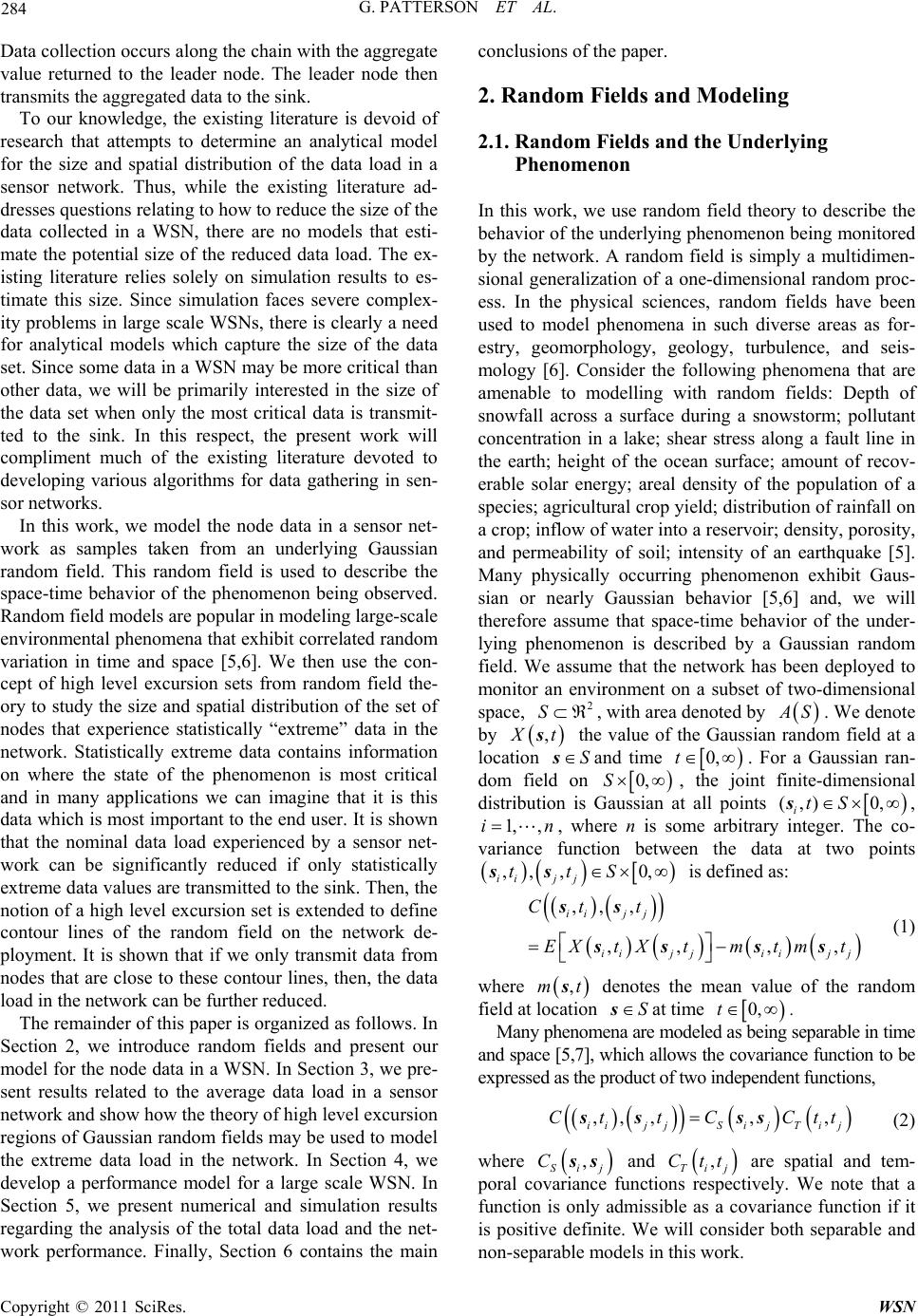

284 G. PATTERSON ET AL.
Data collection occurs along the chain with the aggregate
value returned to the leader node. The leader node then
transmits the aggregated data to the sink.
To our knowledge, the existing literature is devoid of
research that attempts to determine an analytical model
for the size and spatial distribution of the data load in a
sensor network. Thus, while the existing literature ad-
dresses questions relating to how to reduce the size of the
data collected in a WSN, there are no models that esti-
mate the potential size of the reduced data load. The ex-
isting literature relies solely on simulation results to es-
timate this size. Since simulation faces severe complex-
ity problems in large scale WSNs, there is clearly a need
for analytical models which capture the size of the data
set. Since some data in a WSN may be more critical than
other data, we will be primarily interested in the size of
the data set when only the most critical data is transmit-
ted to the sink. In this respect, the present work will
compliment much of the existing literature devoted to
developing various algorithms for data gathering in sen-
sor networks.
In this work, we model the node data in a sensor net-
work as samples taken from an underlying Gaussian
random field. This random field is used to describe the
space-time behavior of the phenomenon being observed.
Random field models are popular in modeling large-scale
environmental phenomena that exhibit correlated random
variation in time and space [5,6]. We then use the con-
cept of high level excursion sets from random field the-
ory to study the size and spatial distribution of the set of
nodes that experience statistically “extreme” data in the
network. Statistically extreme data contains information
on where the state of the phenomenon is most critical
and in many applications we can imagine that it is this
data which is most important to the end user. It is shown
that the nominal data load experienced by a sensor net-
work can be significantly reduced if only statistically
extreme data values are transmitted to the sink. Then, the
notion of a high level excursion set is extended to define
contour lines of the random field on the network de-
ployment. It is shown that if we only transmit data from
nodes that are close to these contour lines, then, the data
load in the network can be further reduced.
The remainder of this paper is organized as follows. In
Section 2, we introduce random fields and present our
model for the node data in a WSN. In Section 3, we pre-
sent results related to the average data load in a sensor
network and show how the theory of high level excursion
regions of Gaussian random fields may be used to model
the extreme data load in the network. In Section 4, we
develop a performance model for a large scale WSN. In
Section 5, we present numerical and simulation results
regarding the analysis of the total data load and the net-
work performance. Finally, Section 6 contains the main
conclusions of the paper.
2. Random Fields and Modeling
2.1. Random Fields and the Underlying
Phenomenon
In this work, we use random field theory to describe the
behavior of the underlying phenomenon being monitored
by the network. A random field is simply a multidimen-
sional generalization of a one-dimensional random proc-
ess. In the physical sciences, random fields have been
used to model phenomena in such diverse areas as for-
estry, geomorphology, geology, turbulence, and seis-
mology [6]. Consider the following phenomena that are
amenable to modelling with random fields: Depth of
snowfall across a surface during a snowstorm; pollutant
concentration in a lake; shear stress along a fault line in
the earth; height of the ocean surface; amount of recov-
erable solar energy; areal density of the population of a
species; agricultural crop yield; distribution of rainfall on
a crop; inflow of water into a reservoir; density, porosity,
and permeability of soil; intensity of an earthquake [5].
Many physically occurring phenomenon exhibit Gaus-
sian or nearly Gaussian behavior [5,6] and, we will
therefore assume that space-time behavior of the under-
lying phenomenon is described by a Gaussian random
field. We assume that the network has been deployed to
monitor an environment on a subset of two-dimensional
space, , with area denoted by
2
S

A
S. We denote
by


,
X
ts
S
the value of the Gaussian random field at a
location

sand time


0,t

. For a Gaussian ran-
dom field on


0,S

, the joint finite-dimensional
distribution is Gaussian at all points


0,tS (,)
i
s,
1,i,n

, where n is some arbitrary integer. The co-
variance function between the data at two points






,, ,
j j
tt 0,S
ii

ss is defined as:






   
,, ,
,, ,,
iij j
iij jiij j
Ct t
EXtXtmt mt



ss
ss ss
(1)
where


,mts denotes the mean value of the random
field at location S

sat time .


0,t
Many phenomena are modeled as being separable in time
and space [5,7], which allows the covariance function to be
expressed as the product of two independent functions,
 



,, ,,,
iij jSijTi j
Ctt CCttss ss

(2)
where


,
Sij
Css and are spatial and tem-
poral covariance functions respectively. We note that a
function is only admissible as a covariance function if it
is positive definite. We will consider both separable and
non-separable models in this work.

,
Tij
Ctt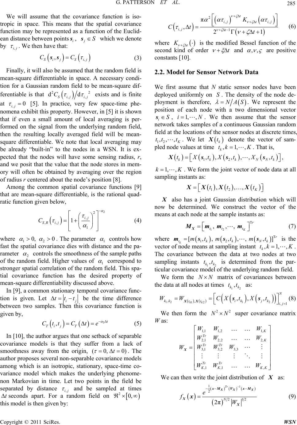


G. PATTERSON ET AL.
285
We will assume that the covariance function is iso-
tropic in space. This means that the spatial covariance
function may be represented as a function of the Euclid-
ean distance between pointsi sj swhich we denote
by ,ij
, S

. then have that: We



,
,
SijSij
CC  ss
(3)
Finally, it will also be assumed that the random field is
mean-square differentiable in space. A necessary condi-
tion for a Gaussian random field to be mean-square dif-
ferentiable is that

2
,,
dd
Sijij
C2

 exists and is finite
at ,0
ij

 [5]. In practice, very few space-time phe-
nomena exhibit this property. However, in [5] it is shown
that if even a small amount of local averaging is per-
formed on the signal from the underlying random field,
then the resulting locally averaged field will be mean-
square differentiable. We note that local averaging may
be already “built-in” to the nodes in a WSN. It is ex-
pected that the nodes will have some sensing radius, r,
and we posit that the value that the node stores in mem-
ory will often be obtained by averaging over the region
of radius r centered about the node’s position [8].
Among the common spatial covariance functions [9]
that are mean-square differentiable, is the rational quad-
ratic function given below,

2
2
,
,,
1
1ij
SR ij
C






 





(4)
where 12 0, 0

 . The parameter 1

controls how
fast the spatial covariance dies with distance and the pa-
rameter 2

controls the smoothness of the sample paths
of the random field. Higher values of 1

correspond to
stronger spatial correlation of the random field. This spa-
tial covariance function has the desired property of
mean-square differentiability discussed above.
In [9], a common stationary temporal covariance func-
tion is given. Let ij
ttt  be the time difference
between two samples. Then this covariance function is
given by,


3
,t
Tij T
CttCt e


 (5)
In [10], the author argues that one setback of separable
covariance models is that they suffer from a lack of
smoothness away from the origin, (0, 0t





2
,,
,1
π
,21
t
ijtij
ij t
K
Ct t



 










  (6)
where


t
K
 

is the modified Bessel function of the
second kind of order t



 and ,,



are positive
constants [10].
2.2. Model for Sensor Network Data
We first assume that N static sensor nodes have been
deployed uniformly on . The density of the node de-
ployment is therefore,
S

NAS  . We represent the
position of each node with a two dimensional vector
iS

s, 1, ,iN


,
. We then assume that the sensor
network takes samples of a continuous Gaussian random
field at the locations of the sensor nodes at discrete times,
12
,,
K
ttt. We let


k
t
k
X
tk
denote the vector of sam-
pled node values at time . That is,
,1,,K






12
,, ,,,,
kkkNN
tXtXtX t

k





Xsss ,
1, ,kK

. We form the joint vector of node data at all
sampling instants as:

 
12
,,,
K
tt t




XX XX
X
also has a joint Gaussian distribution which will
now be determined. We construct the vector of the
means at each node at the sample instants as:
12
T
, ,,
K
r
tt t






X
Mmm m (7)
where




T
12
[,, ,,, ,]r
tkkN
mtmtm tms ss
,1
k
tk
k is the
vector of node means at sampling instant
k
,,K

.
The covariance between the data at two nodes at two
sampling instants 12 is determined from the par-
ticular covariance model of the underlying random field.
,
kk
tt
We form the NN

matrix of covariances between
the data at all nodes at times as:
12
,
kk
tt
 
 


121 2
12
,,,1
,, ,
kk
N
kki kjk tt ij
WW CXtXt






XX ss (8)
We then form the super covariance matrix
W as:
2
NN2
1,1 1,21,
2,1 2,22,
3,13,2 3,3
,1 ,1,
K
Tr
K
Tr Tr
Tr Tr
KK KK
WW W
WW W
WWW W
WW W






















X
)

. The
author proposes several non-separable covariance models
among which is an isotropic, stationary, space-time co-
variance model which makes the underlying phenome-
non Markovian in time. Let two points in the field be
separated by distance ,ij

and be sampled at times
seconds apart. For a random field on
t


0, 
2

this model is then given by:
We can then write the joint distribution of
X
as:



1
1
2
122
2π
Tr W
N
e
f
W

 

XX X
xM xM
X
X
x (9)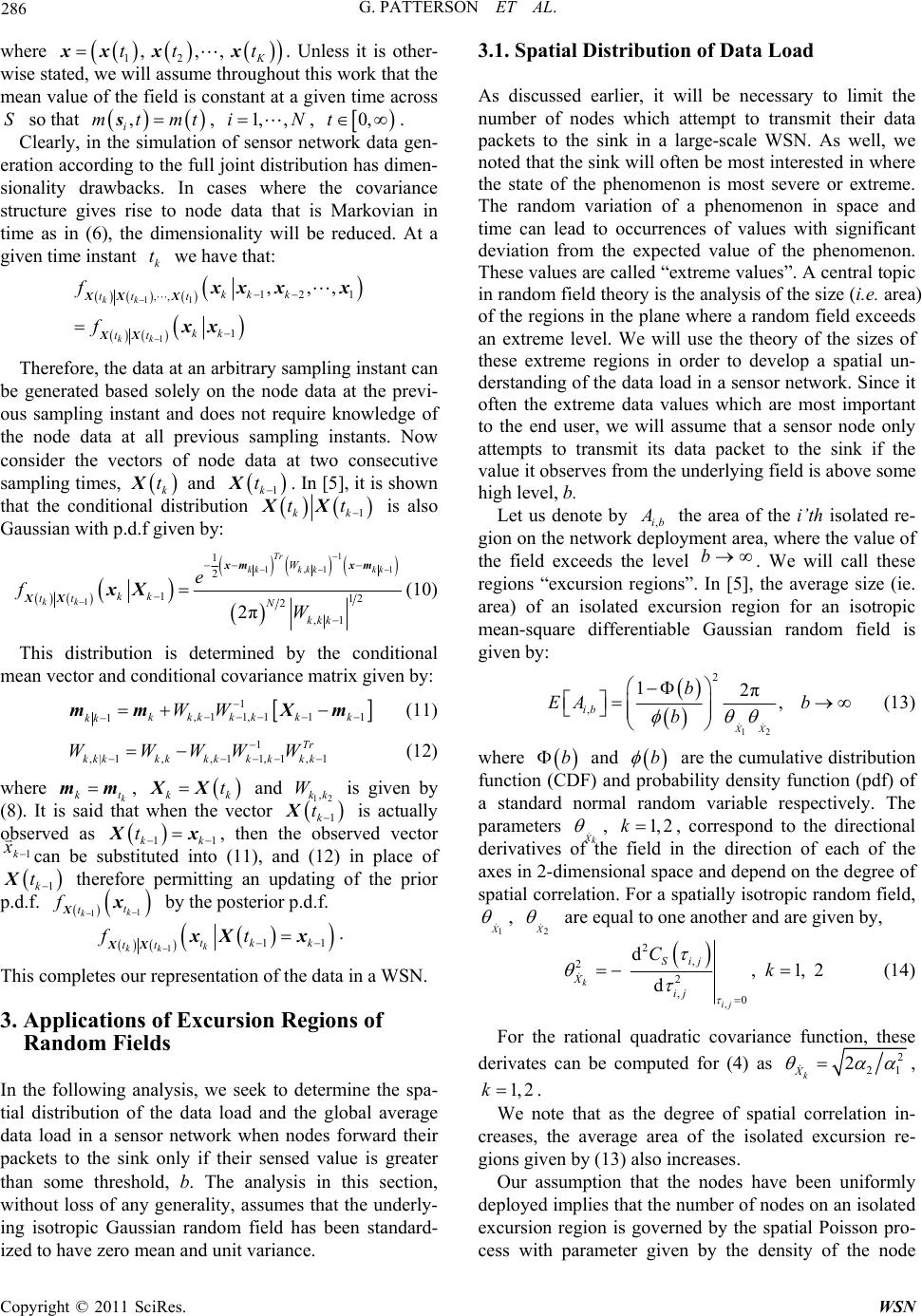

286 G. PATTERSON ET AL.
where . Unless it is other-
wise stated, we will assume throughout this work that the
mean value of the field is constant at a given time across
so that ,
  
12
, ,,
K
tt txx xx
 
,
i
mtmts1, ,SiN

, .
 
0,t
Clearly, in the simulation of sensor network data gen-
eration according to the full joint distribution has dimen-
sionality drawbacks. In cases where the covariance
structure gives rise to node data that is Markovian in
time as in (6), the dimensionality will be reduced. At a
given time instant we have that:
k
t
  

 


11
1
12 1
,,
1
,,,
kk
kk
kk k
tt t
kk
tt
f
f





 XX X
XX
xx xx
xx
Therefore, the data at an arbitrary sampling instant can
be generated based solely on the node data at the previ-
ous sampling instant and does not require knowledge of
the node data at all previous sampling instants. Now
consider the vectors of node data at two consecutive
sampling times, and . In [5], it is shown
that the conditional distribution

k
tX

1k
t X

 
1kk
tt

XX is also
Gaussian with p.d.f given by:
 



1
1,1 1
1
1
2
112
2
,1
2π
Tr
kkk kkkk
kk
W
kk
tt N
kkk
e
f
W



 



xm xm
XX xX

(10)
This distribution is determined by the conditional
mean vector and conditional covariance matrix given by:


1
,1 1,111 1kkkkkkk kk WW

   mm Xm (11)
1
,| 1,,11,1, 1
Tr
kkkkk kkkkkk
WWWWW


 

(12)
where k
kt
, k and is given by
(8). It is said that when the vector is actually
observed as 
mm
t

k
tXX

11kk

12
,kk
W

1k
t X
X
x

, then the observed vector
can be substituted into (11), and (12) in place of
k therefore permitting an updating of the prior
p.d.f. by the posterior p.d.f.
1k
x

tX


1


1k kt
t
f

Xx
1
 



x
111
k
kk tk k
tt
ft

XX xX .
This completes our representation of the data in a WSN.
3. Applications of Excursion Regions of
Random Fields
In the following analysis, we seek to determine the spa-
tial distribution of the data load and the global average
data load in a sensor network when nodes forward their
packets to the sink only if their sensed value is greater
than some threshold, b. The analysis in this section,
without loss of any generality, assumes that the underly-
ing isotropic Gaussian random field has been standard-
ized to have zero mean and unit variance.
3.1. Spatial Distribution of Data Load
As discussed earlier, it will be necessary to limit the
number of nodes which attempt to transmit their data
packets to the sink in a large-scale WSN. As well, we
noted that the sink will often be most interested in where
the state of the phenomenon is most severe or extreme.
The random variation of a phenomenon in space and
time can lead to occurrences of values with significant
deviation from the expected value of the phenomenon.
These values are called “extreme values”. A central topic
in random field theory is the analysis of the size (i.e. area)
of the regions in the plane where a random field exceeds
an extreme level. We will use the theory of the sizes of
these extreme regions in order to develop a spatial un-
derstanding of the data load in a sensor network. Since it
often the extreme data values which are most important
to the end user, we will assume that a sensor node only
attempts to transmit its data packet to the sink if the
value it observes from the underlying field is above some
high level, b.
Let us denote by ,ib
A
the area of the i’th isolated re-
gion on the network deployment area, where the value of
the field exceeds the level . We will call these
regions “excursion regions”. In [5], the average size (ie.
area) of an isolated excursion region for an isotropic
mean-square differentiable Gaussian random field is
given by:
b


12
2
,
12π,
XX
ib
b
EA b
b 








 
(13)
where


b and


b  are the cumulative distribution
function (CDF) and probability density function (pdf) of
a standard normal random variable respectively. The
parameters Xk

, 1, 2k

, correspond to the directional
derivatives of the field in the direction of each of the
axes in 2-dimensional space and depend on the degree of
spatial correlation. For a spatially isotropic random field,
1
X

,
2
X

 are equal to one another and are given by,


,
2
,
2
2
,0
d, 1, 2
d
k
ij
Sij
X
ij
Ck




 
 (14)
For the rational quadratic covariance function, these
derivates can be computed for (4) as 2
21
2
k
X

 
,
1, 2k

.
We note that as the degree of spatial correlation in-
creases, the average area of the isolated excursion re-
gions given by (13) also increases.
Our assumption that the nodes have been uniformly
deployed implies that the number of nodes on an isolated
excursion region is governed by the spatial Poisson pro-
cess with parameter given by the density of the node

G. PATTERSON ET AL.
287
deployment,

NAS  . We call a node whose posi-
tion lies within an isolated excursion region for a given
level b at a sampling time, an “excursion node”. We note
that by virtue of their location, excursion nodes necessar-
ily have a data value exceeding the level b. Let ,ib
K
denote the number of nodes on the excursion re-
gion for extreme value level b. We have that:
' ith


,
,
,
Pr ,
!
ib
kEA
ib
ib
EA e
Kk b
k


 


 
(15)
where we have approximated the area of an excursion
region with its expected value (13). The average number
of nodes on the excursion region is given by: 'ith
,,
,
ib ib
KEAb 


 
(16)
In [5], it is further shown that as the level b increases,
the number of isolated excursion regions approaches a
spatial Poisson process with the parameter given by:

,
1,
b
ib
bb
EA





 (17)
From (17), the rate of isolated excursion regions in the
plane, b

, is inversely proportional to the average area
of an isolated excursion region. Therefore, as the degree
of spatial correlation increases, the frequency of the ex-
cursion regions in the plane decreases proportionately.
Expressions (13) and (17) imply that when the spatial
correlation of the underlying phenomenon is high, the
nodes that observe extreme values will tend to be located
on a relatively small number of large excursion regions.
On the other hand, for low value of spatial correlation,
the nodes that observe extreme values will tend to be
located on a large number of small excursion regions.
The preceding comments offer great insight into the spa-
tial distribution of excursion nodes (equivalently, the
data load) on the network deployment area.
A natural question arises, how high must the level b be
taken so that (13) and (17) hold. In [5], it is recom-
mended that b be at least twice the standard deviation of
the random field. An excellent study on the accuracy of
these expressions for non-asymptotic levels is found in
[11] where the authors look at a random field model de-
scribing the salt-induced delamination of a concrete slab.
3.2. Average Global Data Load
In this section, we derive an expression for the total av-
erage number of nodes which observe data above an ar-
bitrary level, b, and therefore attempt to forward their
data to the sink.
We define the global excursion area as the total area of
the network deployment where

,
X
tbs and denote
this area by b

. In [5] it is shown that for a region with
area 0, the average area within 0 that exceeds b is
given by
a a





01ab when the random field is spa-
tially homogeneous. Since we have assumed that the
underlying phenomenon is spatially isotropic (which
implies homogeneity, see [5,7]), we have that:

 
1AS 


b 

b
 (18)
where


b is the cumulative distribution function
(CDF) of a standard normal random variable. We note
that this expression only depends on the level of the
threshold b and is independent of the spatial correlation
of the random field.
Expression (18) will allow us to determine the total
average data load experienced by a WSN in response to
the sampling of the phenomenon for an arbitrary value b.
Suppose that a sensor node only attempts to send its own
data packet to the sink if the data value in this packet
exceeds the level b. Denote the total number of excursion
nodes in the network by b
K
. Since we have assumed
that the sensor nodes have been uniformly deployed on S
with density

, the average number of excursion nodes
in the network (equivalently, the average number of data
packets or data load) at a sampling time is given by:

1Nb
bb
 K  

 
(19)
This last expression shows that the total average num-
ber of excursion nodes is the same as if the data at the
nodes were i.i.d. This obviously follows from the invari-
ance of b

to the degree of spatial correlation. Thus,
the spatial distribution of the data values according to the
covariance model of the random field has no bearing on
the total average data load. In this respect, this expres-
sion describes the data load only on a global scale over
the whole network and does not capture information on
the location of the excursion nodes themselves. If the
level b is extreme, then the results from Section 3.1 can
be used to gain insight into the spatial description of this
total data load at various regions throughout S will often
be needed in large-scale WSNs.
An ability to describe the spatial distribution of the
data load (as in Section 3.1) will provide insight into
local contention for the channel, the spatial distribution
of newly generated data packets, and the spatial distribu-
tion of energy consumption. The utility of our expression
for the average global data load in (19) is useful from the
perspective that all node data must pass through the in-
formation bottleneck that occurs around the sink in a
WSN [8]. Many characteristic performance measures
will be strongly influenced by the behavior of the net-
work in the region closest to the sink and so, (19) de-
scribes the average data load that the nodes in this region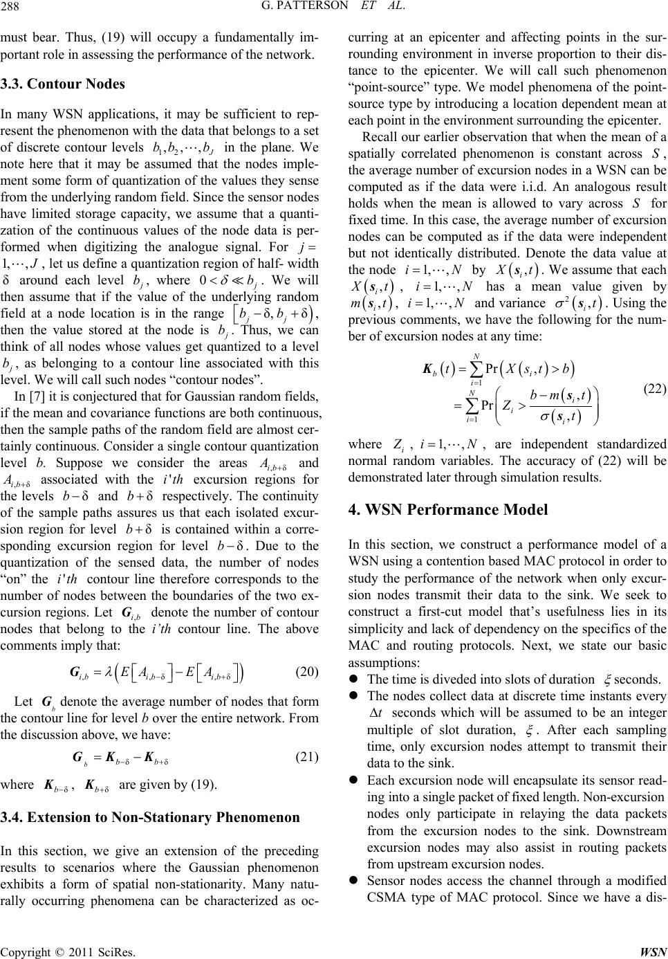

288 G. PATTERSON ET AL.
must bear. Thus, (19) will occupy a fundamentally im-
portant role in assessing the performance of the network.
3.3. Contour Nodes
In many WSN applications, it may be sufficient to rep-
resent the phenomenon with the data that belongs to a set
of discrete contour levels 12
,,,
J
bb b in the plane. We
note here that it may be assumed that the nodes imple-
ment some form of quantization of the values they sense
from the underlying random field. Since the sensor nodes
have limited storage capacity, we assume that a quanti-
zation of the continuous values of the node data is per-
formed when digitizing the analogue signal. For j

1, ,
J

δ
, let us define a quantization region of half- width
around each level
j
b, where 0
j
b



. We will
then assume that if the value of the underlying random
field at a node location is in the range jj
,
then the value stored at the node is

δδ,bb
j
b. Thus, we can
think of all nodes whose values get quantized to a level
j
b, as belonging to a contour line associated with this
level. We will call such nodes “contour nodes”.
In [7] it is conjectured that for Gaussian random fields,
if the mean and covariance functions are both continuous,
then the sample paths of the random field are almost cer-
tainly continuous. Consider a single contour quantization
level b. Suppose we consider the areas ,δib
A

and
,δib associated with the excursion regions for
the levels and respectively. The continuity
of the sample paths assures us that each isolated excur-
sion region for level is contained within a corre-
sponding excursion region for level . Due to the
quantization of the sensed data, the number of nodes
“on” the contour line therefore corresponds to the
number of nodes between the boundaries of the two ex-
cursion regions. Let ,ib denote the number of contour
nodes that belong to the i’th contour line. The above
comments imply that:
A'ith
δb
'
ith
δb
δ b
G
δ
b

,,δ,δibib ib
EA EA 

 

G


δ
(20)
Let bdenote the average number of nodes that form
the contour line for level b over the entire network. From
the discussion above, we have:
G
δ
bbb
GK K (21)
where δb
K
, δb
K
are given by (19).
3.4. Extension to Non-Stationary Phenomenon
In this section, we give an extension of the preceding
results to scenarios where the Gaussian phenomenon
exhibits a form of spatial non-stationarity. Many natu-
rally occurring phenomena can be characterized as oc-
curring at an epicenter and affecting points in the sur-
rounding environment in inverse proportion to their dis-
tance to the epicenter. We will call such phenomenon
“point-source” type. We model phenomena of the point-
source type by introducing a location dependent mean at
each point in the environment surrounding the epicenter.
Recall our earlier observation that when the mean of a
spatially correlated phenomenon is constant across ,
the average number of excursion nodes in a WSN can be
computed as if the data were i.i.d. An analogous result
holds when the mean is allowed to vary across for
fixed time. In this case, the average number of excursion
nodes can be computed as if the data were independent
but not identically distributed. Denote the data value at
the node
S
S
1, ,iN

 by

,
i

X
ts. We assume that each


,
i
X
ts, 1, ,iN

 has a mean value given by


,
i
mts, 1,,iN

 and variance . Using the
previous comments, we have the following for the num-
ber of excursion nodes at any time:

2,
it
 s

 



1
1
Pr ,
,
Pr ,
N
bi
i
Ni
i
ii
tXstb
bmt
Zt












K
s
s
(22)
where , 1,,
i
Z
iN

, are independent standardized
normal random variables. The accuracy of (22) will be
demonstrated later through simulation results.
4. WSN Performance Model
In this section, we construct a performance model of a
WSN using a contention based MAC protocol in order to
study the performance of the network when only excur-
sion nodes transmit their data to the sink. We seek to
construct a first-cut model that’s usefulness lies in its
simplicity and lack of dependency on the specifics of the
MAC and routing protocols. Next, we state our basic
assumptions:
 The time is diveded into slots of duration

seconds.
 The nodes collect data at discrete time instants every
t

seconds which will be assumed to be an integer
multiple of slot duration,

. After each sampling
time, only excursion nodes attempt to transmit their
data to the sink.
 Each excursion node will encapsulate its sensor read-
ing into a single packet of fixed length. Non-excursion
nodes only participate in relaying the data packets
from the excursion nodes to the sink. Downstream
excursion nodes may also assist in routing packets
from upstream excursion nodes.
 Sensor nodes access the channel through a modified
CSMA type of MAC protocol. Since we have a dis-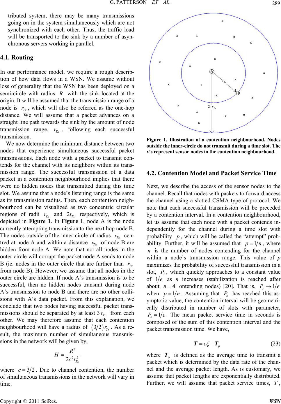

G. PATTERSON ET AL.
289
tributed system, there may be many transmissions
going on in the system simultaneously which are not
synchronized with each other. Thus, the traffic load
will be transported to the sink by a number of asyn-
chronous servers working in parallel.
4.1. Routing
In our performance model, we require a rough descrip-
tion of how data flows in a WSN. We assume without
loss of generality that the WSN has been deployed on a
semi-circle with radius with the sink located at the
origin. It will be assumed that the transmission range of a
node is Tx, which will also be referred as the one-hop
distance. We will assume that a packet advances on a
straight line path towards the sink by the amount of node
transmission range, , following each successful
transmission.
R
Tx
r
r
We now determine the minimum distance between two
nodes that experience simultaneous successful packet
transmissions. Each node with a packet to transmit con-
tends for the channel with its neighbors within its trans-
mission range. The successful transmission of a data
packet in a contention neighbourhood implies that there
were no hidden nodes that transmitted during this time
slot. We assume that a node’s listening range is the same
as its transmission radius. Then, each contention neigh-
bourhood can be visualized as two concentric circular
regions of radii Tx and respectively, which is
depicted in Figure 1. In Figure 1, node A is the node
currently attempting transmission to the next hop node B.
The nodes outside of the inner circle of radius Tx cen-
tred at node A and within a distance Tx of node B are
hidden from node A. We note that not all nodes in the
outer circle will corrupt the packet node A sends to node
B (ie. nodes in the outer circle that are further than Tx
from node B). However, we assume that all nodes in the
outer circle are hidden. If node A’s transmission is to be
successful, then no hidden nodes transmit during node
A’s transmission to node B and there are no other colli-
sions with A’s data packet. From this explanation, we
conclude that two nodes having successful packet trans-
missions should be separated by at least 3Tx from each
other. We may therefore assume that each contention
neighbourhood will have a radius of
r2Tx r
r
r
r
r

32 Tx r. As a re-
sult, the maximum number of simultaneous transmis-
sions in the network will be given by,
2
22
2Tx
R
Hcr 
where 32c. Due to channel contention, the number
of simultaneous transmissions in the network will vary in
time.
Figure 1. Illustration of a contention neighbourhood. Nodes
outside the inner-circle do not transmit during a time slot. The
x’s represent sensor nodes in the contention neighbourhood.
4.2. Contention Model and Packet Service Time
Next, we describe the access of the sensor nodes to the
channel. Recall that nodes with packets to forward access
the channel using a slotted CSMA type of protocol. We
note that each successful transmission will be preceded
by a contention interval. In a contention neighbourhood,
let us assume that each node with a packet contends in-
dependently for the channel during a time slot with
probability , which will be called the “attempt” prob-
ability. Further, it will be assumed that
p
1pn, where
is the number of nodes contending for the channel
within a node’s transmission range. This value of p
maximizes the probability of successful transmission in a
slot,
n
s
P, which quickly approaches to a constant value
of 1e
n
as n increases (stabilization is reached after
about 4

ontending nodes) [20]. That is, 1
s
Pe
when 1pn

. Assuming that
s
P has reached this as-
ymptotic value, the contention interval will be geometri-
cally distributed in number of slots with parameter,
1
s
Pe

. The mean packet service time in seconds is
composed of the sum of this contention interval and the
packet transmission time. We have,
p
e 

TT (23)
where
p
T is defined as the average time to transmit a
packet which is determined by the data rate of the chan-
nel and the average packet length. As is customary, we
assume that packet lengths are exponentially distributed.
Further, we will assume that packet service times, , T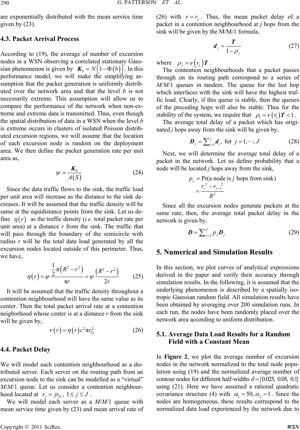

G. PATTERSON ET AL.
290
b 

are exponentially distributed with the mean service time
given by (23).
4.3. Packet Arrival Process
According to (19), the average of number of excursion
nodes in a WSN observing a correlated stationary Gaus-
sian phenomenon is given by . In this
performance model, we will make the simplifying as-
sumption that the packet generation is uniformly distrib-
uted over the network area and that the level b is not
necessarily extreme. This assumption will allow us to
compare the performance of the network when non-ex-
treme and extreme data is transmitted. Thus, even though
the spatial distribution of data in a WSN when the level b
is extreme occurs in clusters of isolated Poisson distrib-
uted excursion regions, we will assume that the location
of each excursion node is random on the deployment
area. We then define the packet generation rate per unit
area as,

1
bN


K

b
A
S
 
K
(24)
Since the data traffic flows to the sink, the traffic load
per unit area will increase as the distance to the sink de-
creases. It will be assumed that the traffic density will be
same at the equidistance points from the sink. Let us de-
fine as the traffic density (i.e. total packet rate per
unit area) at a distance r from the sink. The traffic that
will pass through the boundary of the semicircle with
radius r will be the total data load generated by all the
excursion nodes located outside of this perimeter. Thus,
we have,

r 



22 22
1π
2
π2
Rr Rr
rrr
 


(25)
It will be assumed that the traffic density throughout a
contention neighbourhood will have the same value as its
center. Then the total packet arrival rate at a contention
neigborhood whose center is at a distance r from the sink
will be given by,
 
22
πTx rrc  r
mean service time given by (23) and mean arrival rate of
(26)
4.4. Packet Delay
We will model each contention neighbourhood as a dis-
tributed server. Each server on the routing path from an
excursion node to the sink can be modelled as a “virtual”
M/M/1 queue. Let us consider a contention neighbour-
hood located at . , 1
jTx
rjrjJ
We will model each server as a M/M/1 queue with
(26) with
j
rr

. Thus, the mean packet delay of a
packet in a tion neighbourhood at j hops from the
sink will be given by the M/M/1 formula,
conten
1
j
j


T
d (27)
where


jj r  T.
contention neThe ighbourhoods that a packet passes
through on its routing path correspond to a series of
M/M/1 queues in tandem. The queue for the last hop
which interfaces with the sink will have the highest traf-
fic load. Clearly, if this queue is stable, then the queues
of the preceding hops will also be stable. Thus for the
stability of the system, we require that


11
1r  T.
The average total delay of a packeti- which has orig
na
(28)
Next, we will determine the average total delay of
pa
ted j hops away from the sink will be given by,
, for 1,,
jjJ
Dd
1
ji
i
a
cket in the network. Let us define probability that a
node will be located j hops away from the sink,
22
1
2
Pr(a node is hops from sink)
j
pj
jj
rr
R



Since all the excursion nodes generate packets at the
same rate, then, the average total packet delay in the
network is given by,
J
1
j
j
jp 

D
D (29)
. Numerical and Simulation Results
this section, we plot curves of analytical expressions
.1. Average Data Load Results for a Random
Figure 2, we plot the average number of excursion
5
In
derived in the paper and verify their accuracy through
simulation results. In the following, it is assumed that the
underlying phenomenon is described by a spatially iso-
tropic Gaussian random field. All simulation results have
been obtained by averaging over 200 simulation runs. In
each run, the nodes have been randomly placed over the
network area according to uniform distribution.
5Field with a Constant Mean
In
nodes in the network normalized to the total node popu-
lation using (19) and the normalized average number of
contour nodes for different half-widths


0.025, 0.05, 0.1  
using (21). Here we have assumed a
covariance structure (4) with 12 50, 1
rational quadratic

 . Since the
nodes are homogeneous, theseond to the results corresp
normalized data load experienced by the network due to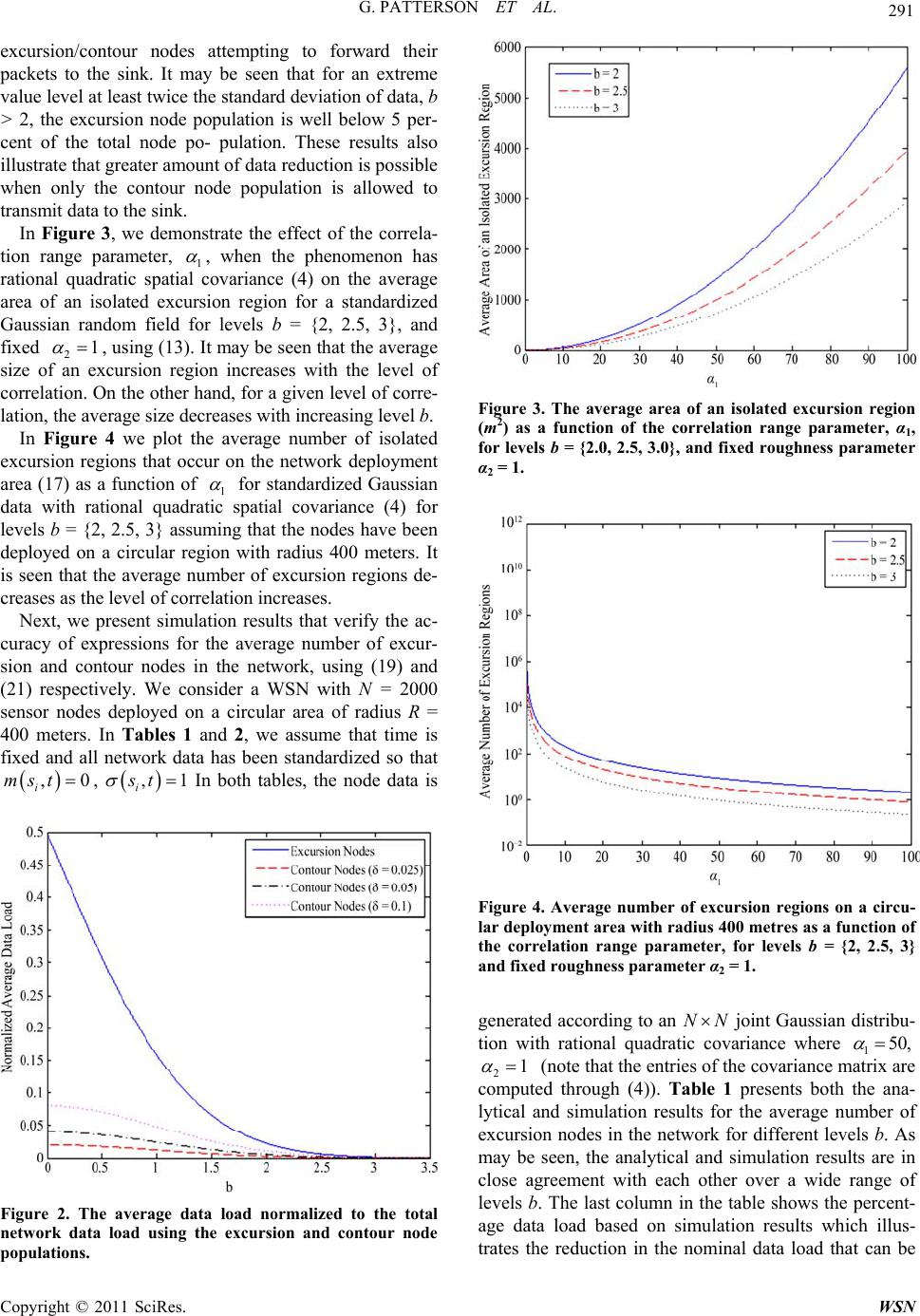

G. PATTERSON ET AL.
291
excursion/contour nodes attempting to forward their
packets to the sink. It may be seen that for an extreme
value level at least twice the standard deviation of data, b
> 2, the excursion node population is well below 5 per-
cent of the total node po- pulation. These results also
illustrate that greater amount of data reduction is possible
when only the contour node population is allowed to
transmit data to the sink.
In Figure 3, we demonstrate the effect of the correla-
tion range parameter, 1

, when the phenomenon has
rational quadratic spatial covariance (4) on the average
area of an isolated excuion region for a standardized
Gaussian random field for levels b = {2, 2.5, 3}, and
fixed 21
rs

, using (13). It may be seen that the average
size of an excursion region increases with the level of
correlan the other hand, for a given level of corre-
lation, the average size decreases with increasing level b.
In Figure 4 we plot the average number of isolated
excursion regions that occur on the network deployment
tion. O
area (17) as a function of 1

for standardized Gaussian
data with rational quadratic spatial covariance (4) for
levels b = {2, 2.5, 3} assumng that the nodes have been
deployed on a circular region with radius 400 meters. It
is seen that the average number of excursion regions de-
creases as the level of correlation increases.
Next, we present simulation results that verify the ac-
curacy of expressions for the average numb
i
er of excur-
si on and contour nodes in the network, using (19) and
(21) respectively. We consider a WSN with N = 2000
sensor nodes deployed on a circular area of radius R =
400 meters. In Tables 1 and 2, we assume that time is
fixed and all network data has been standardized so that

,0
i
mst ,

,1
i
st   In both tables, the node data is
Figure 3. The average area of an isolated excursion region
(m2) as a function of the correlation range parameter, α1
for levels b = {2.0, 2.5, 3.0}, and fixed roughness parameter
,
α2 = 1.
Figure 4. Average number of excursion regions on a circu-
lar deployment area with radius 400 metres as a function of
the correlation range parameter, for levels b = {2, 2.5, 3}
on with rational quadrariance where
and fixed roughness parameter α2 = 1.
generated according to an NN joint Gaussian distribu-
ti tic cova150,


21


(note that the entriee covariance matrix are
computed through (4)). Table 1 presents both the ana-
lytical and simulation results for the average number of
excursion nodes in the network for different levels b. As
may be seen, the analytical and simulation results are in
close agreement with each other over a wide range of
levels b. The last column in the table shows the percent-
age data load based on simulation results which illus-
trates the reduction in the nominal data load that can be
s of th
Figure 2. The average data load normalized to the total
network data load using the excursion and contour node
populations.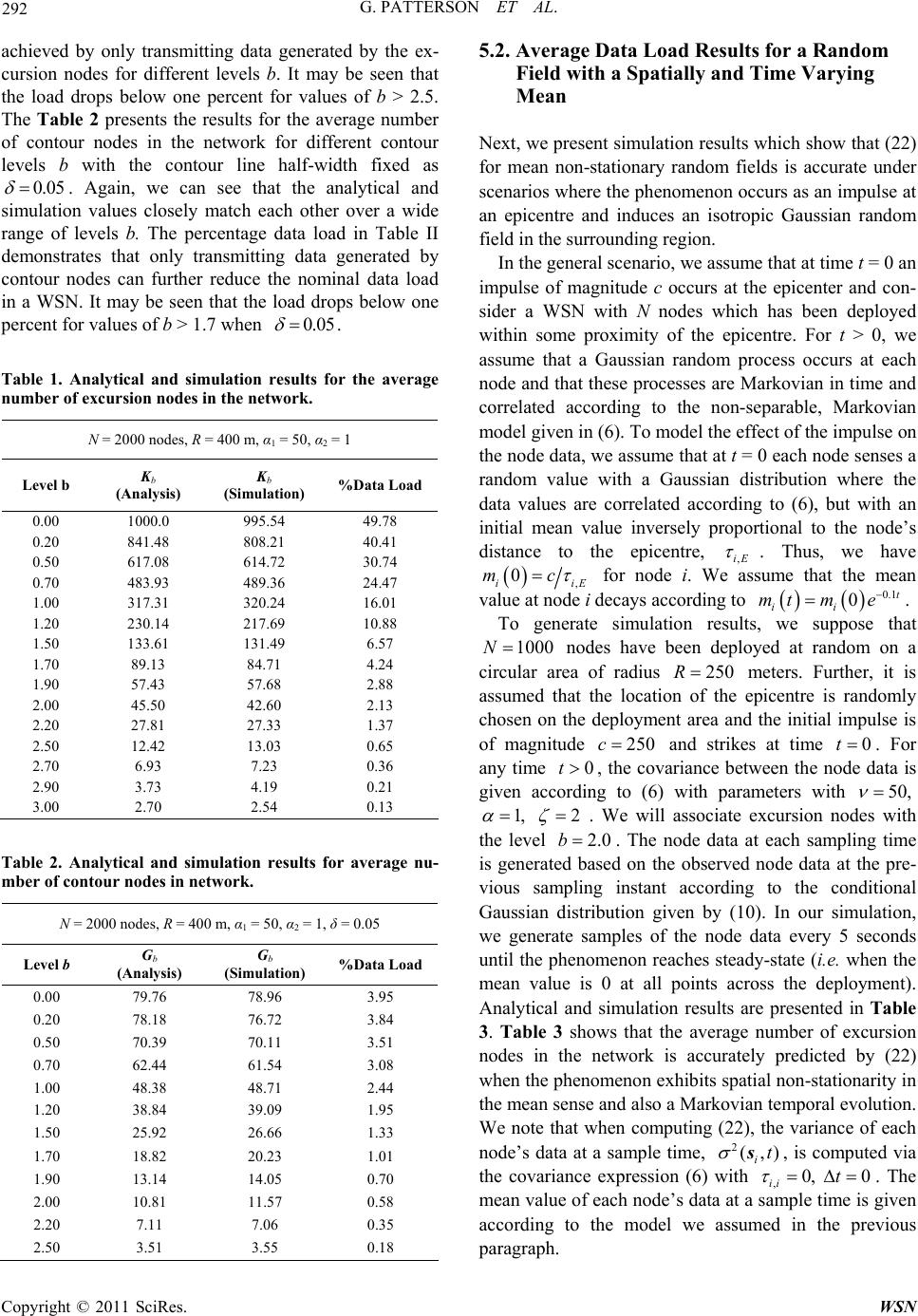

292 G. PATTERSON ET AL.
5.2. Average Data Load Results for a Random
d with atially anime Vary
n
Nex (22)
for m-stationary random fields is accurate under
enarios where the phenomenon occurs as an impulse at
hich has been deployed
w
achieved by only transmitting data generated by the ex-
cursion nodes for different levels b. It may be seen that
the load drops below one percent for values of b > 2.5.
The Table 2 presents the results for the average number
of contour nodes in the network for different contour
levels b with the contour line half-width fixed as
0.0 5

. Again, we can see that the analytical and
simulation values closely match each other over a wide
range of levels b. The percentage data load in Table II
ates that only transmitting data generated by
contour nodes can further reduce the nominal data load
in a WSN. It may be seen that the load drops below one
percent for values of b > 1.7 when 0.05
demonstr

.
Table 1. Analytical and simulation results for the average
number of excursion nodes in the network.
N = 2000 nodes, R = 400 m, α1 = 50, α2 = 1
Level b Kb Kb
(Analysis) (Simulation) %Data Load
0.00 1000.49.78 0 995.54
0.20
0.50
8 841.4808.21 40.41
30.74 617.08 614.72
0.70 483.93 489.36 24.47
1.00 317.31 320.24 16.01
1.20 230.14 217.69 10.88
1.50 133.61 131.49 6.57
1.70 89.13 84.71 4.24
1.90 57.43 57.68 2.88
2.00 45.50 42.60 2.13
2.20 27.81 27.33 1.37
2.50 12.42 13.03 0.65
2.70 6.93 7.23 0.36
2.90 3.73 4.19 0.21
3.00 2.70 2.54 0.13
Table 2. Analytical and simular average nu-
mbeontour nin networ k.
tion results fo
r of codes
N = 2000 nodes, R = 400 m, α1 = 50, α2 = 1, δ = 0.05
Level b Gb G
(Analysis) b (Simulation) %Data Load
0.00 79.76 78.96 3.95
0.20
0.50
Fiela Spd Ting
Mea
t, we present simulation results which show that
ean non
sc
an epicentre and induces an isotropic Gaussian random
field in the surrounding region.
In the general scenario, we assume that at time t = 0 an
impulse of magnitude c occurs at the epicenter and con-
sider a WSN with N nodes w
ithin some proximity of the epicentre. For t > 0, we
assume that a Gaussian random process occurs at each
node and that these processes are Markovian in time and
correlated according to the non-separable, Markovian
model given in (6). To model the effect of the impulse on
the node data, we assume that at t = 0 each node senses a
random value with a Gaussian distribution where the
data values are correlated according to (6), but with an
initial mean value inversely proportional to the node’s
distance to the epicentre, ,iE

. Thus, we have


,
0
iiE
mc

 for node i. We assume that the mean
value at node i decays according to



0.1
0t
ii
mt me

.
To generate simulation res, we suppose that ults
1000N

nodes have been deployed at random on a
circular area of radius 250R

mis eters. Further, it
ass
chosen on
umed that the location of the epicentre is randomly
the deployment area and the initial impulse is
of magnitude 250c

anes at time 0td strik

. For
any time 0t, the covariance between the node data is
given according to (6) with parameters with 50,


1, 2


. l associate excursion nodes with
the level .0
We wil
2b

. The node data at each sampling time
is generated based on the observed node data at the
g instant according to the conditional
Gaussian tion given by (10). In our simulation,
we generate samples of the node data every 5 seconds
until the phenomenon reaches steady-state (i.e. when the
mean value is 0 at all points across the deployment).
Analytical and simulation results are presented in Table
3. Table 3 shows that the average number of excursion
nodes in the network is accurately predicted by (22)
when the phenomenon exhibits spatial non-stationarity in
the mean sense and also a Markovian temporal evolution.
We note that when computing (22), the variance of each
node’s data at a sample time, 2(,)
it
 s, is computed via
the covariance expression (6) with ,0, 0
ii t
pre-
vious sam
d
plin
istribu


. The
mean value of each node’s data at a sample time is given
according to the model we in the previous
paragraph.
778.18 6.72 3.84
3.51 70.39 70.11
0.70 62.44 61.54 3.08
1.00 48.38 48.71 2.44
1.20 38.84 39.09 1.95
1.50 25.92 26.66 1.33
1.70 18.82 20.23 1.01
1.90 13.14 14.05 0.70
2.00 10.81 11.57 0.58
2.20 7.11 7.06 0.35
2.50 3.51 3.55 0.18
assumed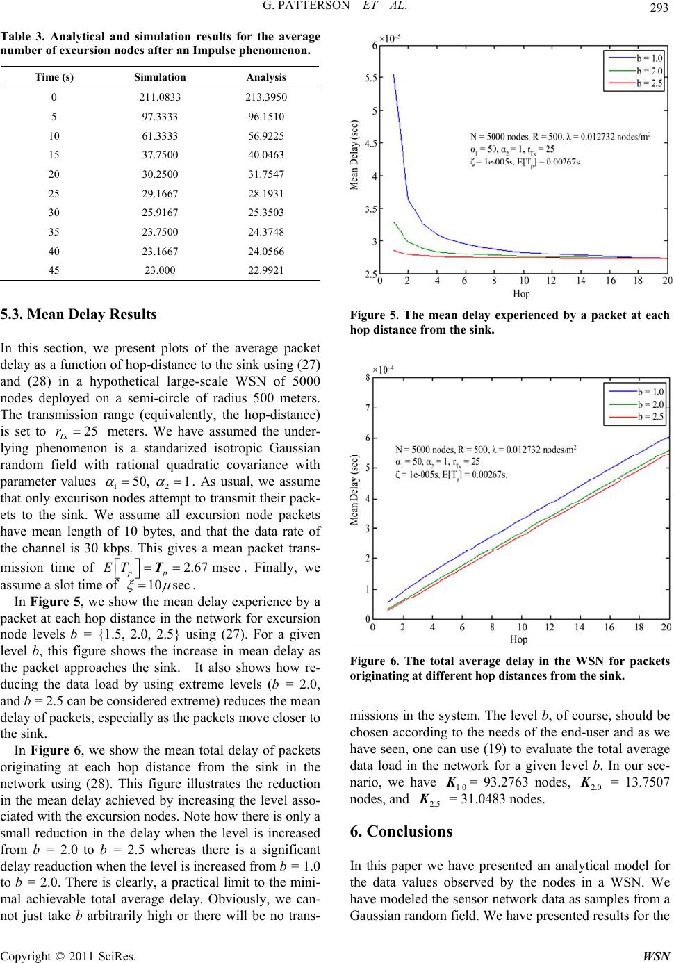

G. PATTERSON ET AL.
293
Table 3. Analytical and simulation results for the average
number of excursion nodes after an Impulse phe nome non.
Time (s) Simulation Analysis
0 211.0833 213.3950
5 97.3333 96.1510
10 61.3333 56.9225
15 37.7500 40.0463
20 30.2500 31.7547
25 29.1667 28.1931
30 25.9167 25.3503
35 23.7500 24.3748
40 23.1667 24.0566
45 23.000 22.9921
5.3. Mean Delay Results
this section, we present plots of the average packet
tance to the sink using (27)
nd (28) in a hypothetical large-scale WSN of 5000
In
delay as a function of hop-dis
a
nodes deployed on a semi-circle of radius 500 meters.
The transmission range (equivalently, the hop-distance)
is set to 25
Tx
r meters. We have assumed the under-
lying phenomenon is a standarized isotropic Gaussian
random field with rational quadratic covariance with
parameter 12 50, 1 values

 . As usual, we assume
that only excurison nodes attempt to transmit their pack-
ets to the sink. We assume all excursion node packets
have mean length nd that the data rate of
the channel is 30 kbps. This gives a mean packet trans-
mission time of 2.67 msec
pp
ET


T. Finally, we
assume a slot time of 10 sec
of 10 bytes, a

 .
In Figure 5, we show the mean delay experience by a
packet at each hopfor excursion distance in the network
2.0, 2.5} ug (27). For a given
le
ng (28). This figure illustrates the reduction
in
not just take b arbitrarily high or there will be no trans-
node levels b = {1.5, sin
vel b, this figure shows the increase in mean delay as
the packet approaches the sink. It also shows how re-
ducing the data load by using extreme levels (b = 2.0,
and b = 2.5 can be considered extreme) reduces the mean
delay of packets, especially as the packets move closer to
the sink.
In Figure 6, we show the mean total delay of packets
originating at each hop distance from the sink in the
network usi
the mean delay achieved by increasing the level asso-
ciated with the excursion nodes. Note how there is only a
small reduction in the delay when the level is increased
from b = 2.0 to b = 2.5 whereas there is a significant
delay readuction when the level is increased from b = 1.0
to b = 2.0. There is clearly, a practical limit to the mini-
mal achievable total average delay. Obviously, we can-
Figure 5. The mean delay experienced by a packet at each
hop distance from the sink.
Figure 6. The total average delay in the WSN for packets
originating at different hop distances from the sink.
missions in the system. The level b, of course, should be
verage
ata load in the network for a given level b. In our sce-
chosen according to the needs of the end-user and as we
have seen, one can use (19) to evaluate the total a
d
nario, we have 1.0
K
= 93.2763 nodes, 2.0
K
= 13.7507
nodes, and 2.5
K
= 31.0483 nodes.
6. Conclusions
In this pape have presented an r weanalytical model for
e data values observed by the nodes in a WSN. We
nsor network data as samples from a
aussian random field. We have presented results for the
th
have modeled the se
G

G. PATTERSON ET AL.
294
tour Maps:
Monitoring and Diagnosis in Sensor Networks,” Com-
s: the International Journal of Computer
unication Networking (ACM), Vol. 50, No.
average total area of the network that experiences data
above an arbitrary level b, and the average area of an
isolated excursion region containing extreme data when
the level b is chosen sufficiently high. It has been shown
that the number of excursion regions on the network de-
ployment approaches a Poisson distribution for extreme
levels, b. The average size of the isolated excursion re-
gions increases while their frequency decreases when the
level of spatial correlation is increased. It has also been
observed that the sum of the average size of excursion
regions and the average excursion node population for a
level b are a function of b alone and not on the degree of
spatial correlation. We have quantified the data reduction
that may be achieved by only transmitting data from ex-
cursion and contour nodes for various levels b. Finally, a
performance model has been presented for large-scale
sensor networks that can be used to derive the mean de-
lay experienced by packets at each hop on their journey
to the sink. The results of the paper will be useful in the
design of large sensor networks in ensuring that the net-
work meets the requirements of the end user.
7. References
[1] X. Meng and T. Nandagopal, et.al. “Con
puter Network
and Telecomm
15, 2006, pp. 2820-2838.
doi:10.1016/j.comnet.2005.09.038
[2] S. R. Madden, M. J. Franklin, J. M. Hellerstein and W.
Hong, “TAG: A Tiny Aggregation Service for Ad-Hoc Sen-
sor Networks”, Proceedings of OSDI, Boston, June 2002.
[3] S. Yoon and C. Shahabi, “The Clustered AGgregation
(CAG) Technique Leveraging Spatial and Temporal
Correlations in Wireless Sensor Networks,” ACM Trans-
actions on Sensor Networks, Vol. 3, No. 1, article No. 3,
March, 2007. doi:10.1145/844128.844142
[4] S. Lindsey and K. M. Sivalingam, “Data Gathering Algo-
rithms in Sensor Networks Using Energy Metrics,” IEEE
Transactions on Parallel and Distributed Systems. Vol.
13, No. 9, 2002, pp. 924-934.
doi:10.1109/TPDS.2002.1036066
[5] E. Vanmarcke, “Random Fields: Analysis and Synthesis,”
iley Encyclopedia of Sta-
n Random Fields
. Willig, “Protocols and Architectures For
ral
MIT Press, Cambridge, 1983.
[6] R. Adler, “Random Fields,” W
tistical Sciences, 2006.
http://www.mrw.interscience.wiley.com/emrw/97804716
67193/ess/article/ess2164/current/html
[7] P. Abrahamsen, “A Review of Gaussia
and Correlation Functions,” 2nd Edition, Norwegian
Computing Center, April 1997.
http://www.math.ntnu.no/~omre/TMA4250/V2007/abrah
amsen2.ps.
[8] H. Karl, A
Wireless Sensor Networks,” Wiley, New York, 2005.
[9] M. Vuran, O. Akan and I. Akyildiz, “Spatio-Tempo
Correlation: Theory and Applications for Wireless Sensor
Networks,” Computer Networks, Vol. 45, No. 3, 2004, pp.
245-259. doi:10.1016/j.comnet.2004.03.007
[10] M. Stein, “Space-Time Covariance Functions,” Journal
of American Statistical Association, Vol. 100, No. 469,
2005, pp. 310-321.
doi:10.1198/016214504000000854
[11] G. A. Fenton, “A Random Field Excursion Model of
Salt-Induced Concrete Delamination,” Journal of Re-
search of the National Institute of Standards and Tech-
nology, Vol. 99, No. 4, 1994, pp. 475-483.
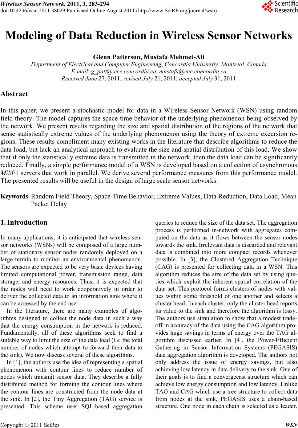