Open Access Library Journal
Vol.03 No.05(2016), Article ID:69338,10 pages
10.4236/oalib.1102620
Solar Sail Equilibrium Orbits in the Circular Restricted Three-Body Problem with Oblateness
Ming Song*, Xingsuo He, Yehao Yan, Dongsheng He
Northwestern Polytechnical University, Xi’an, China

Copyright © 2016 by authors and OALib.
This work is licensed under the Creative Commons Attribution International License (CC BY).
http://creativecommons.org/licenses/by/4.0/


Received 31 March 2016; accepted 27 May 2016; published 31 May 2016

ABSTRACT
We investigate solar sail in the circular restricted three-body problem, where the larger primary is a source of radiation and the smaller primary is an oblate spheroid in the system. Firstly, the differential equations of motion for solar sail in the system combined effects of radiation and oblateness of celestial bodies are built. Then the positions of the solar sail collinear Lagrange points are calculated as mass ratio or oblateness changes in certain extent. Linearization near the collinear equilibria of the system is applied. A linear quadratic regulator is used to stabilize the nonlinear system. Three different cases of solar sail equilibrium orbits are studied each with different choices for the weight matrices. The simulations reveal that solar sail equilibrium orbits can be stable under active control by changing three angles, incident angle, cone angle and clock angle of the solar sail.
Keywords:
Solar Sail, Restricted Three-Body Problem, Equilibrium Orbits, Oblateness
Subject Areas: Aerospace Engineering

1. Introduction
The solar sail has become a hot topic of research during the last few decades [1] - [5] . It uses sunlight to generate propulsion in space by reflecting solar photon flux from a large, mirror-like sail made of lightweight, highly reflective polyimide film material. Especially after the successful flight of the Interplanetary Kite-craft Accelerated by Radiation of the Sun (IKAROS) in 2010 [6] , a number of new space missions using a solar sail have been proposed, such as NanoSail-D [7] , Cubesail [8] , DeorbitSail [9] and Sunjammer [10] . The reason why the solar sail has increasingly attracted the world’s attention is that, when compared with conventional spacecraft, it can accelerate continually without a propellant. It is this very characteristic that makes the solar sail to execute a few novel space missions that conventional spacecraft could not execute very well; for instance: Solar Polar Imager, Heliostorm, Interstellar Probe and Near Earth Asteroid Rendezvous [11] .
The restricted three-body problem (RTBP) has been considered a basic dynamic model ever since the scientists have studied the solar sail [12] [13] . The RTBP describes the motion of an infinitesimal mass, usually a satellite, solar sail or asteroid, moving under the gravitational effect of two finite masses, normally called primaries, which move in circular orbits about their center of mass under their mutual attraction [5] . Usually we do not take into account of the effect of the infinitesimal mass of the motion of the primaries. However, an absolute spherical celestial body is very rare in space, most of the planets are oblate. Sharma and Rao [14] investigated the locations of the five equilibrium points by considering the effect of oblateness of the more massive primary. Sharma [15] [16] discussed the existence of periodic orbits in the RTBP when the more massive primary was an oblate spheroid. Douskos [17] [18] focused on the equilibrium points and their stability in the Hill’s problem with oblateness. Singh [19] analyzed the combined effects of perturbations, oblateness, and radiation of the primaries on the nonlinear stability of the Lagrange points. However, the above literatures did not take account of the impacts of oblateness on solar sail orbits in RTBP. Solar sail as one of new important deep space probes must be considered the influences of oblateness of celestial bodies if it could observe and study well in the long-term space missions. Therefore, the effects of the oblateness of the primaries should be included when we establish the model of solar sail RTBP and investigate the motion of the solar sail in the RTBP. Thus we achieve better simulation results, which can provide an optimal design for the flight path of the solar sail.
This paper is organized as follows. Section 2 introduces the equations of motion of the system in the circular restricted three-body problem with the larger primary, a source of radiation and the smaller primary, an oblate spheroid. In Section 3, we investigate the equilibrium points of the system with the variations of lightness number of solar sail oroblateness of the smaller primary. Then, in Section 4, linearization near the collinear Lagrange points is taken into account, and the linear quadratic regulator (LQR) is developed to stabilize the nonlinear system. The simulation is given in Section 5. The conclusions are discussed in Section 6.
2. Equations of Motion
The restricted three-body problem with the larger primary a source of radiation and the smaller primary an oblate spheroid is investigated. We use a barycentric, rotating and dimensionless coordinate system Oxyz; the origin is at the barycenter of the primaries; the axis x is along the line joining with the primaries; the direction of the orbital angular velocity ω of the smaller primary defines the axis z; and the axis y completes the right-handed triad. We describe the circular restricted three-body problem in Figure 1. For convenience the dimensionless form is often used [20] . The two primaries have masses m1 and m2 respectively, the mass of the infinitesimal body, the solar sail, is m3. The distance between the primaries is , and the gravitational constant is chosen to be unity. When it comes to the RTBP, the unit mass, length, and time of the system are defined as
 (1)
(1)

Figure 1. Schematic geometry of the circular restricted three-body problem.
Then, in this system the masses of two primaries are ,
,  , where μ is the mass ratio for the system,
 . The distances of two primaries to the barycenter are
 ,
, .
.
Considering the oblateness of the smaller primary, the equations of motion of the solar sail in the rotating coordinate system can be written as
 (2)
(2)
 (3)
(3)
 (4)
(4)
where Ω is the pseudo-potential function [18]
 (5)
(5)
Ωx, Ωy, Ωz are the components of the partial derivative of the pseudo-potential function Ω on each coordinate
axis;  and
and  are the distances of the solar sail from the primaries respectively, and
  is the perturbed mean motion of the primaries; β is the lightness num-
ber of the solar sail.  is the oblateness coefficient of the smaller primary, where RE and RP are the equatorial and polar radii of the smaller primary, and R is the distance between the two primaries [21] . ax, ay, az are the projections of the acceleration produced by the solar radiation pressure force on the axis Ox, Oy, Oz. Figure 2 is a flat solar sail model, where
  is the angle between n (vectors are expressed by black italicized letters in this article) and incident light r1 from larger primary; φ is the cone angle between the projection of n in xy plane; γ is the clock angle between the projection of n in xy plane and xz plane. The acceleration produced by solar radiation pressure force can be expressed [5]
 (6)
(6)
3. Collinear Equilibrium Points
The equilibrium points of the system are the solutions of the equations
 (7)
(7)
 (8)
(8)
 (9)
(9)

Figure 2. A flat solar sail model.
where
 (10)
(10)
 (11)
(11)
 . (12)
We suppose that three collinear equilibrium points  lie on the axis x, then we use
  to denote the collinear equilibria. These collinear Lagrange points satisfy Equations (7), (8) and (9)
 (13)
(13)
 (14)
(14)
 . (15)
According to Equations (13)-(15), we find that collinear equilibrium points will be get when φ and γ equal zero, that is to say, when the surface of solar sail is perpendicular to the radiate light, Equation (13) has effective solution. From Equation (13) we see that the position of collinear equilibrium points varies with the magnitude of the mass ratio μ, oblateness A and lightness number β. In the following, we set μ = 0.001, then the positions of L1, L2, L3 varying with the variations of A and β are shown in Figure 3. It is clear that these collinear equilibrium points are unstable. The effects of oblateness of smaller primary on L1, L2 are obvious, but it has little impact on L3.


Figure 3. Positions of L1, L2, L3 vary with the variations of A and β.
4. Linearization near the Collinear Equilibria
To further investigate the characteristics of the solar sail orbit in the circular restricted three-body problem with oblateness, we need to linearize the system because the differential equations are nonlinear. Given that the collinear Lagrange points of the nonlinear system are , we introduce small perturbations such that we define Equations (16), (17), and (18)
 (16)
(16)
 (17)
(17)
 . (18)
Substitute Equations (16), (17), and (18) into Equations (2), (3) and (4), and assume that the sail acceleration is constant under the small perturbation from the collinear equilibrium point [22] [23] ; then we obtain the variational equations
 (19)
(19)
 (20)
(20)
 (21)
(21)
where
 (22)
(22)
 (23)
(23)
 (24)
(24)
 . (25)
Therein  is the evaluation of the second order partial derivative of the potential function at the equilibrium points. With this method we can get the linear dynamic model and establish its state-space equation expressed in matrix notation as Equation (26)
 (26)
(26)
where the six-dimensional state vector is defined , and
, and
 . (27)
The LQR controller is developed to stabilize the nonlinear system in the neighborhood of the collinear libration point. We apply a linear feedback control  to Equation (26) that minimizes the quadratic cost function
 (28)
(28)
where the matrices Q and R represent the weights of the state and control, which are symmetric positive semidefinite and free to be chosen. We obtain the gain matrix  by solving the algebraic Riccati equation [24]
 . (29)
The closed-loop system is then obtained as
 . (30)
A necessary and sufficient condition for the collinear equilibrium points to be linearly stable is that the real part of the eigenvalues of the matrix A − BK are all less than or equal to zero [25] .
5. Simulation
In this section, we choose μ = 0.001, A = 0.001, β = 0.05 as basic parameters, and as an example, we set initial conditions as ,
,  ,
,  ,
,  ,
,  ,
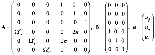
,  , the time of simulation is 15 units time. Three different cases of solar sail equilibrium point orbits are displayed in Figure 4(a), Figure 6(a) and Figure 8(a), and each case has a different choice of weight matrices Q and R, which are elaborated in Table 1.
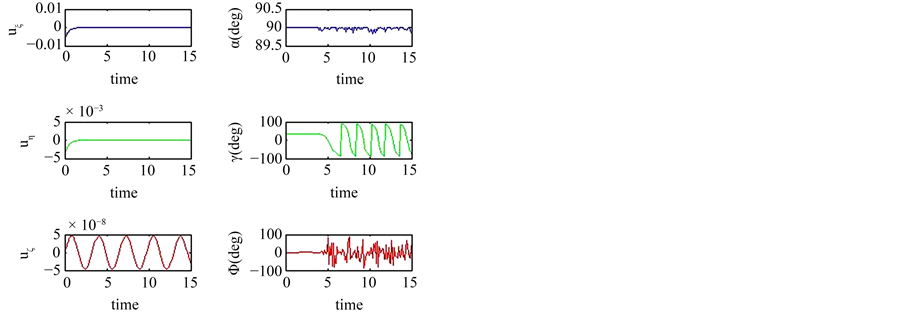
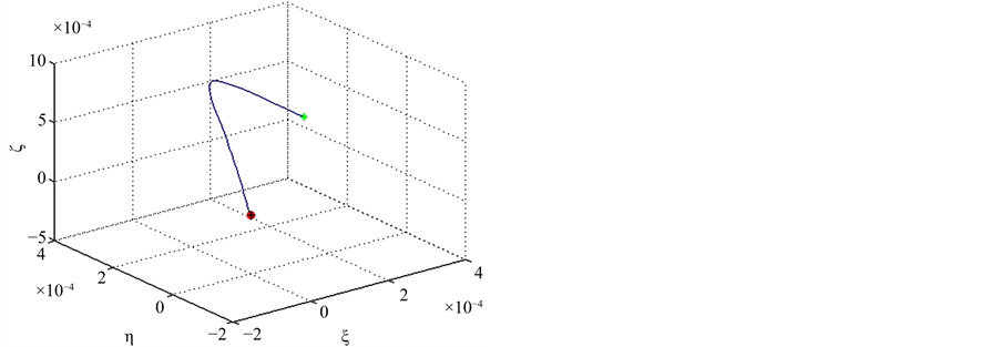
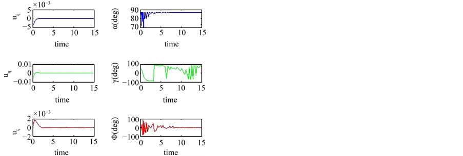
Figure 4(a) is a spiral orbit of the sail in the vicinity of L1. L1 is a sink of this system, small perturbation near the collinear Lagrange point L1 will be asymptotic stable. In Figure 4(b), the left parts are the time curve graphs of projections of solar radiation pressure acceleration on each axis. The projections on ξ and η change mildly and approach zeroquickly. But axis ζ’sprojection changes as a sine curve; the amplitude gets smaller and smaller. The right parts are the variations of three angles, where  is about between 56.3˚ and 90˚, −90˚ ≤ γ, f ≤ 90˚.
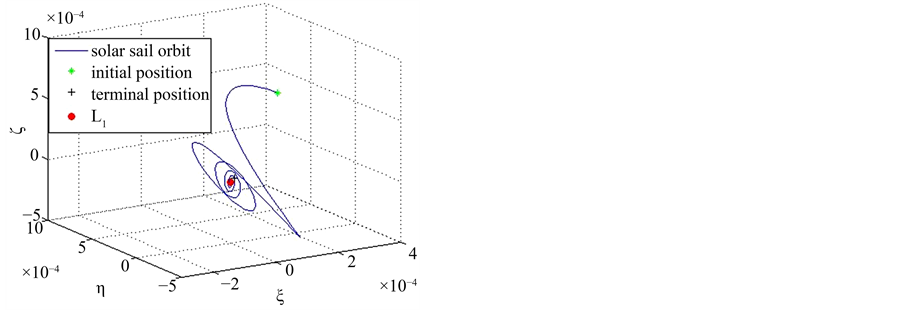
Different from Case A, Figure 6(a1) is the Quasiperiodic orbits of the sail, which are also asymptotic stable. But these kinds of orbits will not come close to L1, just like Figure 6(a2) shown, these quasiperiodic motion will last forever. In Figure 6(b), the left parts, the projections on ξ and η change like those in Case A; the projection on axis ζ changes as a sine curve and the amplitude remains about the same. The right parts are the variations of three angles, where  changes in a small scale about from 89.8˚ to 90˚, −90˚ ≤ γ, f ≤ 90˚. Figure 8(a) displays a direct perturbation trajectory of the sail derived from L1 point. The maximum acceleration of solar radiation pressure is about 0.009906 units acceleration. The minimum
  is about 56.5˚, the maximum
  is 90˚. Meanwhile, the position and velocity of the sail in the vicinity of L1 varying with time are shown in Figure 5, Figure 7
 (a) (b)
Figure 4. (a) The spiral orbit of the sail in the vicinity of L1. (b) Time histories of components of the acceleration of the sail and α, γ, φ the pitch angle in case A.
 (a) (b)
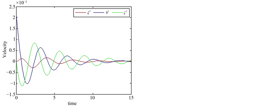
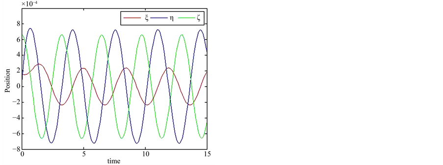
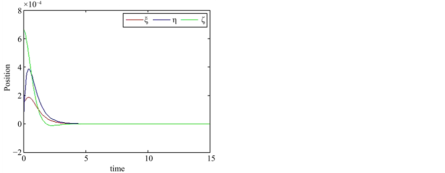
Figure 5. (a) Position modification derived from the solar sail about the L1 point; (b) Velocity change as time increases in case A.

 (a2) (b)
Figure 6. (a1) Quasiperiodic orbits of the sail derived from L1 point in 15 units time; (a2) Quasiperiodic orbits of the sail derived from L1 point in 150 units time; (b) In 15 units time, components of the acceleration of the sail and the pitch angle in case B.
 (a) (b)
Figure 7. (a) Position modification derived from the solar sail about the L1 point; (b) Velocity change as time increases in case B.
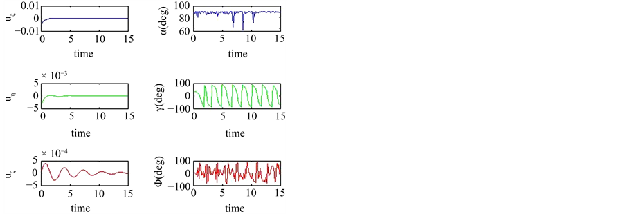
and (k)(l). The minimum and maximum quantitative values of them are displayed in Table 2. In case A the position and velocity swing back and forth and the amplitudes become smaller. In case B cyclical variations are reflected in the position and velocity, which show that the quasiperiodic orbits of the sail are asymptotically stable. However, in case C position and velocity fluctuate dramatically during about the first four units time; after that they change only slightly near the collinear equilibrium point (Figures 4-9).
In Table 1, we have chosen the weighting matrices Q and R and evaluated the gain matrix K and the eigenvalue of matrix A − BK in three different cases. It is quite clear that the real parts of the six eigenvalues of matrix A − BK in all three cases are negative numbers.

Table 1. Parameters for simulation.
 (a) (b)
Figure 8. (a) Direct perturbation trajectory of the sail derived from L1 point; (b) Time histories of components of the acceleration of the sail and the pitch angle in case C.
 (a) (b)
Figure 9. (a) Position modification derived from the solar sail about the L1 point; (b) Velocity change as time increases in case C.
Table 2. Positions and velocity interval of solar sail in three cases.
6. Conclusion
In this paper, we investigate the solar sail equilibrium orbits in the circular restricted three-body problem with oblateness. We find that oblateness has little impact on the position of L3. An LQR controller is used to obtain the numerical solution of the components of solar radiation pressure acceleration. We solve Equation (25) to get the changing laws of angles of the sail, which can make the system stable near the collinear Lagrange points. We can choose different weight matrices Q and R to obtain different solar sail orbits for different space mission requirements.
Cite this paper
Ming Song,Xingsuo He,Yehao Yan,Dongsheng He, (2016) Solar Sail Equilibrium Orbits in the Circular Restricted Three-Body Problem with Oblateness. Open Access Library Journal,03,1-10. doi: 10.4236/oalib.1102620
References
- 1. Tsu, T.C. (1959) Interplanetary Travel by Solar Sail. ARS Journal, 29, 422-427.
http://dx.doi.org/10.2514/8.4791 - 2. Morrow, E., Scheeres, D.J. and Lubin, D. (1978) Solar Sail Orbit Operations at Asteroids. Journal of Spacecraft and Rockets, 38, 279-286.
http://dx.doi.org/10.2514/2.3682 - 3. McInnes, C.R. and Simmons, J.F.L. (1992) Solar Sail Halo Orbits. Part I—Heliocentric Case. Journal of Spacecraft and Rockets, 29, 466-471.
http://dx.doi.org/10.2514/3.25487 - 4. McInnes, C.R. and Simmons, J.F.L. (1992) Solar Sail Halo Orbits Part II—Geocentric Case. Journal of Spacecraft and Rockets, 29, 472-479.
http://dx.doi.org/10.2514/3.55639 - 5. McInnes, C.R. (1999) Solar Sailing: Technology, Dynamics and Mission Applications. Springer Praxis, London.
http://dx.doi.org/10.1007/978-1-4471-3992-8 - 6. Tsuda, Y., Mori, O., Funase, R., Sawada, H., Yamamoto, T., Saiki, T., Endo, T. and Kawaguchi, J. (2011) Flight Status of IKAROS Deep Space Solar Sail Demonstrator. Acta Astronautica, 69, 833-840.
http://dx.doi.org/10.1016/j.actaastro.2011.06.005 - 7. Johnson, L., Whorton, M., Heaton, A., Pinson, R., Laue, G. and Adams, C. (2011) Nanosail-D: A Solar Sail Demonstration Mission. Acta Astronautica, 68, 571-575.
http://dx.doi.org/10.1016/j.actaastro.2010.02.008 - 8. Lappas, V., Adeli, N., Visagie, L., Fernandez, J., Theodorou, T., Steyn, W. and Perren, M. (2011) CubeSail: A Low Cost CubeSat Based Solar Sail Demonstration Mission. Advances in Space Research, 48, 1890-1901.
http://dx.doi.org/10.1016/j.asr.2011.05.033 - 9. Olive, R.S. and Vaios, L. (2013) Deorbitsail: A Deployable Sail for De-Orbiting. 54th AIAA/ASME/ASCE/AHS/ASC Structures, Structural Dynamics, and Materials Conference, Boston, 8 April 2013.
http://dx.doi.org/10.2514/6.2013-1806 - 10. Jeannette, H., Ben, D. William, D. and Colin, M. (2014) Sunjammer: Preliminary End-to-End Mission Design. AIAA/AAS Astrodynamics Specialist Conference, San Diego, California, USA, 4-7 August 2014.
http://dx.doi.org/10.2514/6.2014-4127 - 11. Johnson, L., Swartzlander, G. and Artusio-Glimpse, A. (2014) An Overview of Solar Sail Propulsion within NASA. In: Macdonald, M., Ed., Advances in Solar Sailing, Springer, Berlin Heidelberg, 15-23.
http://dx.doi.org/10.1007/978-3-642-34907-2_2 - 12. Baoyin, H. and McInnes, C. (2006) Solar Sail Equilibria in the Elliptical Restricted Three-Body Problem. Journal of Guidance Control and Dynamics, 29, 538-543.
http://dx.doi.org/10.2514/1.15596 - 13. McInnes, C.R., McDonald, A.J.C., Simmons, J.F.L. and MacDonald, E.W. (2004) Solar Sail Parking in Restricted Three-Body Systems. Journal of Guidance, Control, and Dynamics, 17, 399-406.
http://dx.doi.org/10.2514/3.21211 - 14. Sharma, R.K. and Rao, P.V.S. (1976) Stationary Solutions and Their Characteristic Exponents in the Restricted Three-Body Problem When the More Massive Primary Is an Oblate Spheroid. Celestial Mechanics, 13, 137-149.
http://dx.doi.org/10.1007/BF01232721 - 15. Sharma, R.K. (1976) Periodic Orbits of 1st Kind in Restricted 3-Body Problem When More Massive Primary Is an Oblate Spheroid. Astronomy & Astrophysics, 50, 257-258.
- 16. Sharma, R.K. (1990) Periodic-Orbits of the 3rd Kind in the Restricted 3-Body Problem with Oblateness. Astrophysics and Space Science, 166, 211-218.
http://dx.doi.org/10.1007/BF01094894 - 17. Markakis, M.P., Perdiou, A.E. and Douskos, C.N. (2008) The Photo Gravitational Hill Problem with Oblateness: Equilibrium Points and Lyapunov Families. Astrophysics and Space Science, 315, 297-306.
http://dx.doi.org/10.1007/s10509-008-9831-6 - 18. Douskos, C. and Markellos, V. (2006) Out-of-Plane Equilibrium Points in the Restricted Three-Body Problem with Oblateness. Astronomy & Astrophysics, 446, 357-360.
http://dx.doi.org/10.1051/0004-6361:20053828 - 19. Singh, J. (2009) Combined Effects of Oblateness and Radiation on the Nonlinear Stability of L4 in the Restricted Three-Body Problem. The Astronomical Journal, 137, 3286-3292.
http://dx.doi.org/10.1088/0004-6256/137/2/3286 - 20. Szebehely, V. (1967) Theory of Orbits: The Restricted Problem of Three Bodies. Academic Press, New York.
- 21. Sharma, R.K. and Rao, P.V.S. (1978) A Case of Commensurability Induced by Oblateness. Celestial Mechanics, 18, 185-194.
http://dx.doi.org/10.1007/BF01228715 - 22. Simo, J. and McInnes, C.R. (2009) Solar Sail Orbits at the Earth-Moon Libration Points. Communications in Nonlinear Science and Numerical Simulation, 14, 4191-4196.
http://dx.doi.org/10.1016/j.cnsns.2009.03.032 - 23. Gong, S.P., Li, J.F. and Simo, J. (2014) Orbital Motions of a Solar Sail around the L2 Earth-Moon Libration Point. Journal of Guidance Control and Dynamics, 37, 1349-1356.
http://dx.doi.org/10.2514/1.G000063 - 24. Wie, B. (1998) Space Vehicle Dynamics and Control. AIAA Inc., Reston, Virginia.
- 25. Biggs, J.D. and Mcinnes, C.R. (2010) Passive Orbit Control for Space-Based Geo Engineering. Journal of Guidance Control & Dynamics, 33, 1017-1020.
http://dx.doi.org/10.2514/1.46054
NOTES

*Corresponding author.