Journal of Signal and Information Processing, 2011, 2, 211-217
doi:10.4236/jsip.2011.23029 Published Online August 2011 (http://www.SciRP.org/journal/jsip)
211
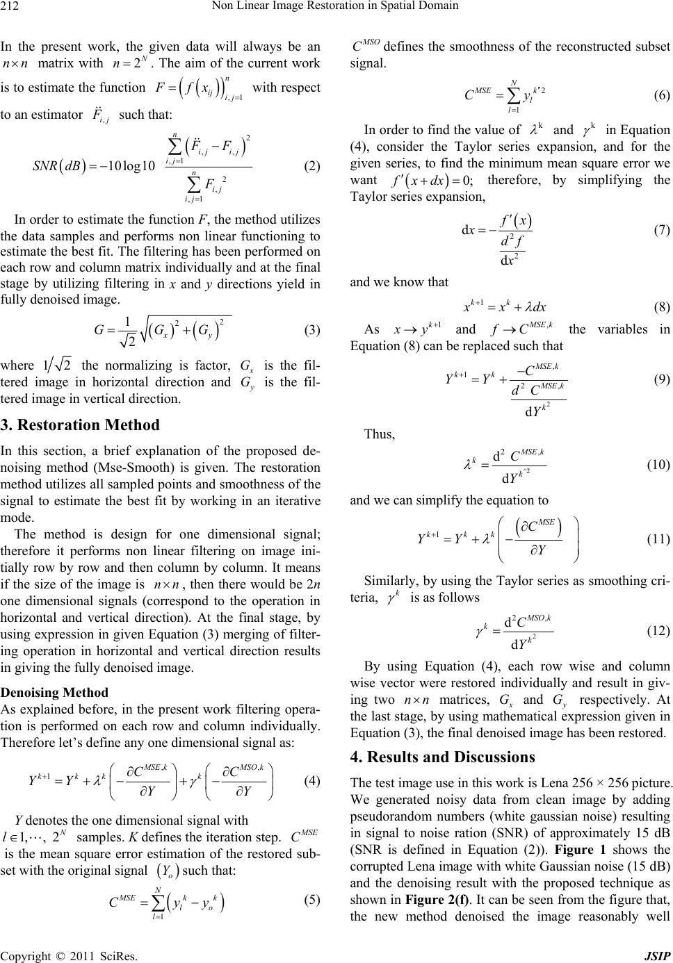
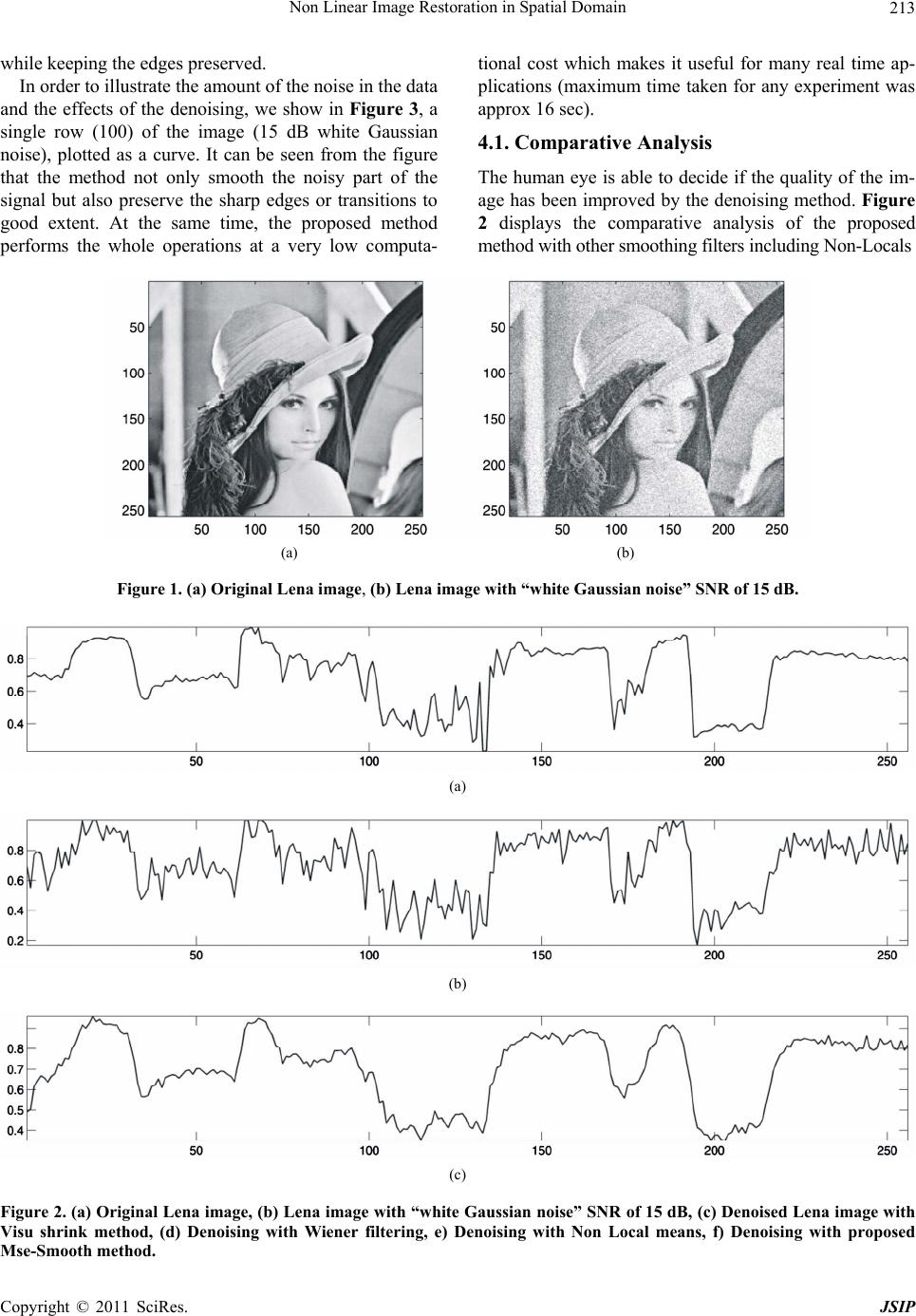
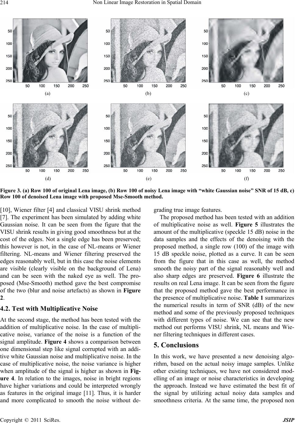
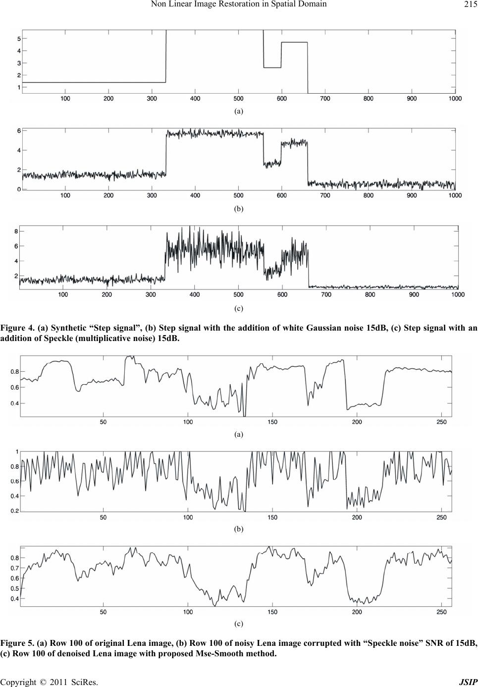
Non Linear Image Restoration in Spatial Domain
Bushra Jalil, Fauvet Eric, Laligant Olivier
Le2i Laboratory, Universite de Bourgogne, Le Creusot, France.
Received May 10th, 2011; revised June 22nd, 2011; accepted July 30th, 2011.
ABSTRACT
In the present work, a novel image restoration method from noisy data samples is presented. The restoration was per-
formed by using some heuristic approach utilizing data samples and smoo thness criteria in spatial domain . Unlike most
existing techniques, this approach do es n ot require p rio r mode lling o f eith er the image or noise statistics. The p roposed
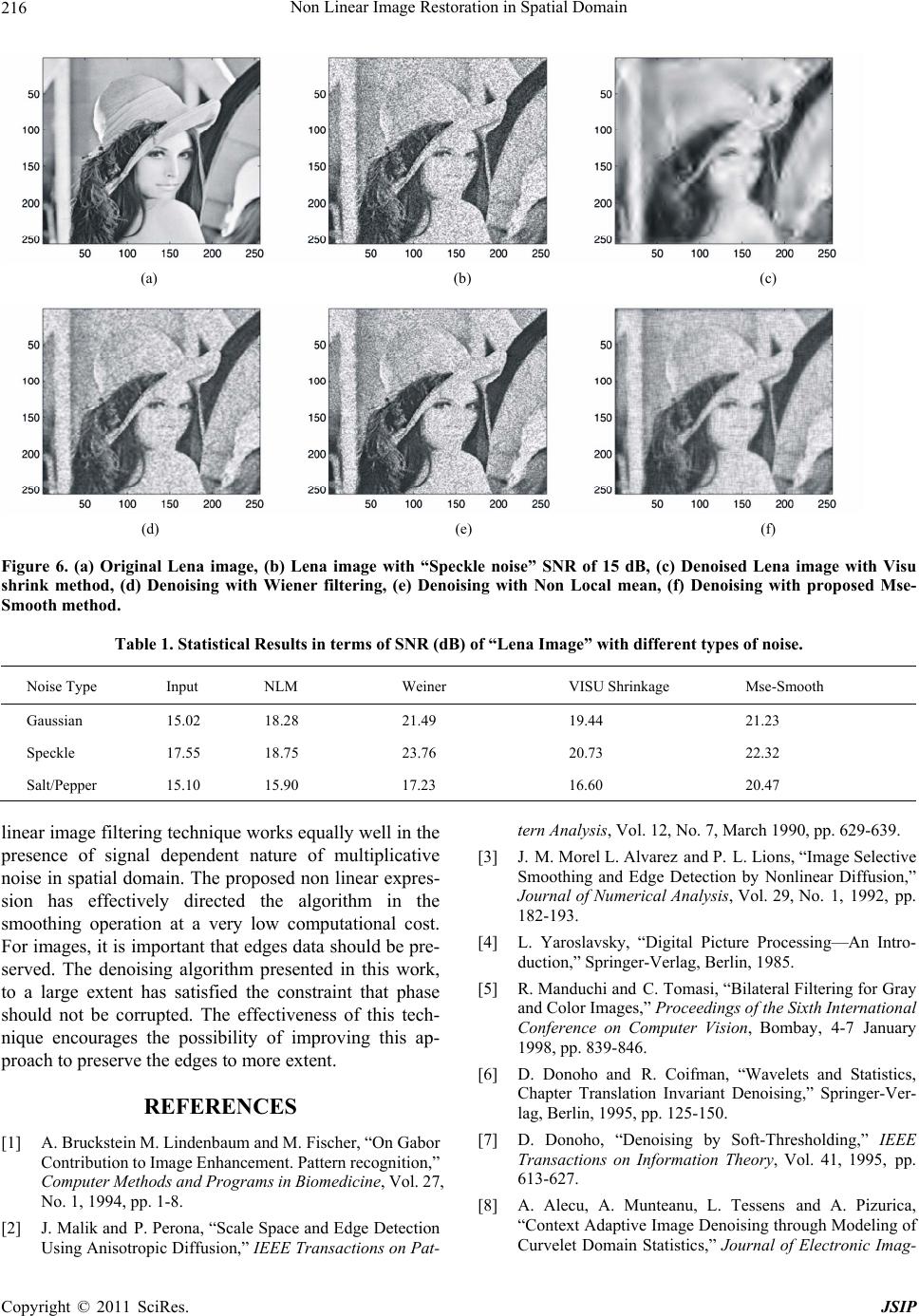
method works in an interactive mode to find the best compromise between the data (mean square error) and the
smoothing criteria. The method has been compared with the shrinkage approach, Wiener filter and Non Local Means
algorithm as well. Experimental results showed that the proposed method gives better signal to noise ratio as compared
to the previously proposed denoising solutions. Furthermore, in addition to the wh ite Gaussian noise, the effectiveness
of the proposed techn ique has also been proved in the presence of multiplicative noise.
Keywords: Restoration, Nonlinear Filtering, Mean Square Error, Signal Smoothness
1. Introduction
The recovery of a signal fro m observed no isy data, while
still preserving its important features, continues to re-
main a fundamentally elusive challenging problem in
signal and image processing. More importantly, the need
for an efficient image restoration method has grown with
the massive production of digital images of different
types. The two main limitations in any image accuracy
are categorized as blur and noise. The main objective of
any filtering method is to effectively suppress the noise
elements.
Not only that, it is of extreme importance to preserve
and enhance the edges at the same time. Several methods
have been proposed in the past to attain these objectives
and to recover the original (noise free) image. Most of
these techniques uses averaging filter e.g. the Gaussian
smoothing model has been used by Gabor [1], some of
these techniques uses anisotropic filtering [2,3] and the
neighbourhood filtering [4,5] and some works in fre-
quency domain e.g. Wiener filters [4]. In the past few
years, wavelet transform has also been used as a signifi-
cant tool to denoise the signal [6-8]. A brief survey of
some of these approaches is given by Buades et al. [9].
Since the scope of this work is limited to spatial domain,
therefore the proposed method has been compared with
the classical methods for denoising in spatial domain.
Traditionally, linear models have been used to extract
the noise elements e.g. Gaussian filter as they are com-
putationally less expensive. However, in most of the
cases the linear models are not able to preserve sharp
edges which are later recognized as discontinu ities in the
image. On the other hand, nonlinear models can effec-
tively handle this task (preserve edges) but more often,
non linear model are computationally expensive. In the
present work, we attempt to propose a non linear model
with the very less computational cost to restore image
from noisy data samples. The method utilizes data sam-
ples and find the best compromise between the data
samples and smoothness criteria which ultimately result
in giving the denoise signal at a very low computational
cost. We have also presented the comparative analysis of
the present technique with some of the previously pro-
posed method.
The paper is organized as follows. The principle of the
proposed technique is given in Section 2. Section 3 ex-
plains the overview of the restoration method. Applica-
tion on images and comparative analysis is given in Sec-
tion 4 and finally Section 5 concludes the work with
some future perspectives.
2. Principle of the Method
We assume that the given data specify the model:


where ,1,,
ijij ij
yfx ij n (1)
f is the noise free signal, uniformly sampled (e.g., an
image) and ij

is the white Gaussian noise


2
0,N

.

Non Linear Image Re st oration in Spatia l Domain 212
In the present work, the given data will always be an
matrix with nn
2
N
n
ij
. The aim of the current work
is to estimate the function with respect
 
,1
n
ij ij
Ffx  
to an estimator ,
F
 such that:


2
,,
,1
2
,
,1
10log10
n
ij ij
ij
n
ij
ij
FF
SNR dBF







(2)
In order to estimate the function F, the method utilizes
the data samples and performs non linear functioning to
estimate the best fit. The filtering has been performed on
each row and column matrix individually and at the final
stage by utilizing filtering in x and y directions yield in
fully denoised image.
 
2
2
1
2xy
GGG (3)
where 12 the normalizing is factor,
x
G is the fil-
tered image in horizontal direction and
y
G is the fil-
tered image in vertical direction.
3. Restoration Method
In this section, a brief explanation of the proposed de-
noising method (Mse-Smooth) is given. The restoration
method utilizes all sampled points and smoothness of the
signal to estimate the best fit by working in an iterative
mode.
The method is design for one dimensional signal;
therefore it performs non linear filtering on image ini-
tially row by row and then column by column. It means
if the size of the image is , then there would be 2n
one dimensional signals (correspond to the operation in
horizontal and vertical direction). At the final stage, by
using expressio n in given Equation (3) merging of filter-
ing operation in horizontal and vertical direction results
in giving the fully denoised image.
nn
Denoising Method
As explained before, in the present work filtering opera-
tion is performed on each row and column individually.
Therefore let’s define any one dimensional signal as:
,
1,
M
SE kMSO k
kkk k
CC
YY YY 


 






(4)
Y denotes the one dimensional signal with
samples. K defines the iteration step. 1,l, 2N 
M
SE
C
is the mean square error estimation of the restored sub-
set with the original signal such that:

o
Y
N

1
M
SO
Cdefines the smoothness of the reconstructed subset
signal.
2
1
N
M
SE k
l
l
Cy


 (6)
In order to find the value of k

and k

in Equation
(4), consider the Taylor series expansion, and for the
given series, to find the minimum mean square error we
want


0;fxdx


 therefore, by simplifying the
Taylor series expansion,

2
2
d
d
f
x
xdf
x

 (7)
and we know that
1kk
x
xdx

 (8)
As 1k
x
y

 and ,
M
SE k
fC the variables in
Equation (8) can be replaced such that
2
,
12
d
,
M
SE k
kk
M
SE k
k
C
YY
dC
Y

 (9)
Thus,
^2
2,
d
d
M
SE k
k
k
C
Y
  (10)
and we can simplify the equation to

1
MSE
kkkC
YY Y 



 
 



(11)
Similarly, by using the Taylor series as smoothing cri-
teria, k

is as follows
2
2,
d
d
M
SO k
k
k
C
Y
  (12)
By using Equation (4), each row wise and column
wise vector were restored individually and result in giv-
ing two nn

matrices,
x
G and
y
G respectively. At
the last stage, by using mathematical expression given in
Equation (3), the final denoised image has been restored.
4. Results and Discussions
The test image use in this work is Lena 256 × 256pictur e.
We generated noisy data from clean image by adding
pseudorandom numbers (white gaussian noise) resulting
in signal to noise ration (SNR) of approximately 15 dB
(SNR is defined in Equation (2)). Figure 1 shows the
corrupted Lena image with white Gaussian noise (15 dB)
and the denoising result with the proposed technique as
shown in Figure 2(f). It can be seen from the figure that,
the new method denoised the image reasonably well

M
SEk k
lo
l
Cy


y
(5)

Non Linear Image Re st oration in Spatia l Domain 213
while keeping the edges preserved.
In order to illustrate the amount of the noise in the data
and the effects of the denoising, we show in Figure 3, a
single row (100) of the image (15 dB white Gaussian
noise), plotted as a curve. It can be seen from the figure
that the method not only smooth the noisy part of the
signal but also preserve the sharp edges or transitions to
good extent. At the same time, the proposed method
performs the whole operations at a very low computa-
tional cost which makes it useful for many real time ap-
plications (maximum time taken for any experiment was
approx 16 sec).
4.1. Comparative Analysis
The human eye is able to decide if the quality of the im-
age has been improved by the denoising method. Figure
2 displays the comparative analysis of the proposed
method with other smoothing filters including Non-Locals
(a) (b)
Figure 1. (a) Original Lena image, (b) Lena image with “white Gaussian noise” SNR of 15 dB.
(a)
(b)
(c)
Figure 2. (a) Original Lena image, (b) Lena image with “white Gaussian noise” SNR of 15 dB, (c) Denoised Lena image with
Visu shrink method, (d) Denoising with Wiener filtering, e) Denoising with Non Local means, f) Denoising with proposed
Mse-Smooth method.

Non Linear Image Re st oration in Spatia l Domain 214
(a) (b) (c)
(d) (e) (f)
Figure 3. (a) Row 100 of original Lena image, (b) Row 100 of noisy Lena image with “white Gaussian noise” SNR of 15 dB, c)
Row 100 of denoised Lena image with proposed Mse-Smooth method.
[10], Wiener filter [4] and classical VISU shrink method
[7]. The experiment has been simulated by adding white
Gaussian noise. It can be seen from the figure that the
VISU shrink results in giving good smoothness but at the
cost of the edges. Not a single edge has been preserved;
this however is not, in the case of NL-means or Wiener
filtering. NL-means and Wiener filtering preserved the
edges reasonably well, but in this case the noise elements
are visible (clearly visible on the background of Lena)
and can be seen with the naked eye as well. The pro-
posed (Mse-Smooth) method gave the best compromise
of the two (blur and noise artefacts) as shown in Figure
2.
4.2. Test with Multiplicative Noise
At the secon d stage, th e method has been tested with the
addition of multiplicative noise. In the case of multipli-
cative noise, variance of the noise is a function of the
signal amplitude. Figure 4 shows a comparison between
one dimensional step like signal corrupted with an addi-
tive white Gaussian noise and multiplicative noise. In the
case of multiplicative noise, the noise variance is higher
when amplitude of the signal is higher as shown in Fig-
ure 4. In relation to the images, noise in bright regions
have higher variations and could be interpreted wrongly
as features in the original image [11]. Thus, it is harder
and more complicated to smooth the noise without de-
grading true image features.
The proposed method has been tested with an addition
of multiplicative noise as well. Figure 5 illustrates the
amount of the multiplicative (speckle 15 dB) noise in the
data samples and the effects of the denoising with the
proposed method, a single row (100) of the image with
15 dB speckle noise, plotted as a curve. It can be seen
from the figure that in this case as well, the method
smooth the noisy part of the signal reasonably well and
also sharp edges are preserved. Figure 6 illustrate the
results on real Lena image. It can be seen from the figure
that the proposed method gave the best performance in
the presence of multiplicative noise. Table 1 summarizes
the numerical results in term of SNR (dB) of the new
method and some of the previously proposed techniques
with different types of noise. We can see that the new
method out performs VISU shrink, NL means and Wie-
ner filtering techniques in different cases.
5. Conclusions
In this work, we have presented a new denoising algo-
rithm, based on the actual noisy image samples. Unlike
other existing techniques, we have not considered mod-
elling of an image or noise characteristics in developing
the approach. Instead we have estimated the best fit of
the signal by utilizing actual noisy data samples and
smothness criteria. At the same time, the proposed non o

Non Linear Image Re st oration in Spatia l Domain215
(a)
(b)
(c)
Figure 4. (a) Synthetic “Step signal”, (b) Step signal with the addition of white Gaussian noise 15dB, (c) Step signal with an
addition of Speckle (multiplicative noise) 15dB.
(a)
(b)
(c)
Figure 5. (a) Row 100 of original Lena image, (b) Row 100 of noisy Lena image corrupted with “Speckle noise” SNR of 15dB,
(c) Row 100 of denoised Lena image with proposed Mse-Smooth method.

Non Linear Image Re st oration in Spatia l Domain 216
(a) (b) (c)
(d) (e) (f)
Figure 6. (a) Original Lena image, (b) Lena image with “Speckle noise” SNR of 15 dB, (c) Denoised Lena image with Visu
shrink method, (d) Denoising with Wiener filtering, (e) Denoising with Non Local mean, (f) Denoising with proposed Mse-
Smooth method.
Table 1. Statistical Results in terms of SNR (dB) of “Lena Image” with different types of noise.
Noise Type Input NLM Weiner VISU Shrinkage Mse-Smooth
Gaussian 15.02 18.28 21.49 19.44 21.23
Speckle 17.55 18.75 23.76 20.73 22.32
Salt/Pepper 15.10 15.90 17.23 16.60 20.47
linear image filtering technique works equally well in the
presence of signal dependent nature of multiplicative
noise in spatial domain. The proposed non linear expres-
sion has effectively directed the algorithm in the
smoothing operation at a very low computational cost.
For images, it is important that edges data should be pre-
served. The denoising algorithm presented in this work,
to a large extent has satisfied the constraint that phase
should not be corrupted. The effectiveness of this tech-
nique encourages the possibility of improving this ap-
proach to preserve the edges to more extent.
REFERENCES
[1] A. Bruckstein M . Lind enbaum and M. Fischer, “On Gabor
Contribution to Imag e Enhancem ent. Pa ttern re cogniti on,”
Computer Methods and Programs in Biomedicine, Vol. 27,
No. 1, 1994, pp. 1-8.
[2] J. Malik and P. Perona, “Scale Space and Edge Detection
Using Anisotropic Diffusion,” IEEE Transactions on Pat-
tern Analysis, Vol. 12, No. 7, March 1990, pp. 629-639.
[3] J. M. Morel L. Alvarez and P. L. Lions, “Image Selective
Smoothing and Edge Detection by Nonlinear Diffusion,”
Journal of Numerical Analysis, Vol. 29, No. 1, 1992, pp.
182-193.
[4] L. Yaroslavsky, “Digital Picture Processing—An Intro-
duction,” Springer-Verlag, Berlin, 1985.
[5] R. Manduchi and C. Tomasi, “Bilateral Filtering for Gray
and Color Images,” Proceedings of the Sixth International
Conference on Computer Vision, Bombay, 4-7 January
1998, pp. 839-846.
[6] D. Donoho and R. Coifman, “Wavelets and Statistics,
Chapter Translation Invariant Denoising,” Springer-Ver-
lag, Berlin, 1995, pp. 125-150.
[7] D. Donoho, “Denoising by Soft-Thresholding,” IEEE
Transactions on Information Theory, Vol. 41, 1995, pp.
613-627.
[8] A. Alecu, A. Munteanu, L. Tessens and A. Pizurica,
“Context Adaptive Image Denoising through Modeling of
Curvelet Domain Statistics,” Journal of Electronic Imag-

Non Linear Image Re st oration in Spatia l Domain217
ing, Vol. 17, No. 3, 2008, p. 033021.
doi:10.1117/1.2987723
[9] J. Morel, A. Buades and B. Coll, “On Image Denoising
Methods,” Technical Report CMLA, 2004.
[10] J. M. Morel, A. Buades and B. Coll, “A Non-Local Algo-
rithm for Image Denoising,” IEEE Computer Society
Conference on Computer Vision and Pattern Recognition,
San Diego, 20-26 June 2005, pp. 60-65.
[11] A. Reza and Y. Hawwar, “Spatially Adaptive Multiplica-
tive Noise Image Denoising Technique,” IEEE Transac-
tions on Image Processing, Vol. 11, No. 12, 2002, pp.
1397-1404. doi:10.1109/TIP.2002.804526