Received 17 February 2016; accepted 3 March 2016; published 8 March 2016

ABSTRACT

The paper investigates the non-local property of quantum mechanics by analyzing the role of the quantum potential in generating the non-local dynamics and how they are perturbed in presence of noise. The resulting open quantum dynamics much depend by the strength of the Hamiltonian interaction: Weakly bounded systems may not be able to maintain the quantum superposition of states on large distances and lead to the classical stochastic evolution. The stochastic hydrodynamic quantum approach shows that the wave-function collapse to an eigenstates can be described by the model itself and that the minimum uncertainty principle is compatible with the relativistic postulate about the light speed as the maximum velocity of transmission of interaction. The paper shows that the Lorenz invariance of the quantum potential does not allow super- luminal transmission of information in measurements on quantum entangled states.

Keywords:

quantum Non-locality, superluminal Transmission of Quantum information, classical Freedom, Local relativisticcausality, EPR Paradox, macroscopic quantum Decoherence

Subject Areas: Modern Physics

1. Introduction

The quantum to classical transition is one of the unsolved problems of the modern physics [1] - [3] . The disconnection between the two theories leaves open the question about the hierarchy between them. The quantum mechanics, on the base of its statistical postulates, needs the classical mechanics (i.e., the classical observer) but it seems to be the basic theory from which the classical mechanics can stem in the macroscopic limit where tends to zero.

One current of thought is represented by the “deterministic” approach to the quantum mechanics that analyzes how the quantum equations are a generalization of the classical one [4] - [13] where the nonlocality is introduced in various ways, the Madelung quantum potential [6] - [8] , the Nelson’s osmotic potential, the Bohm-Hylei quantum potential or the Paris and Wu fifth-time parameter.

The non-local restrictions of the quantum hydrodynamic analogy (QHA) [6] - [8] derive from the application of the quantization of vortices [8] and by the elastic-like energy of the quantum pseudo-potential but not from boundary conditions as happens for the Schrödinger equation where the non-local character of evolution is determined by the initial and boundary conditions that are not included into the equation.

The deterministic approach continuously gains interest in the physics community due to the fact that it helps in explaining quantum phenomena that cannot be easily described by the standard formalism. They are: The multiple tunneling [14] , critical phenomena at zero temperature [15] , mesoscopic physics [16] [17] , numerical solution of the time-dependent Schrödinger equation [18] - [20] , quantum dispersive phenomena in semiconductors [21] , quantum field theoretical regularization procedure [22] and the quantization of Gauge fields, without gauge fixing and without ensuing the Faddeev-Popov ghost [23] .

On the theoretical point of view, one of the most promising aspects of these models is helping in investigating the quantum mechanical problems using efficient mathematical technique such as the stochastic calculus, the numerical approach and supersymmatry.

A parallel current of thought, investigates the possibility of obtaining the classical state through the loss of quantum coherence of classically chaotic systems due to the presence of stochastic fluctuations [24] - [28] . Most of the outputs of this field of investigation are based on numerical simulations or semi-empirical approaches but they do not own a global theoretical view. The quantum decoherence is achieved as a consequence of the chaoticity of motion equations where, due to a high Lyapunov exponent, the future state of the system is very sensitive to a very small fluctuation. In this case the future form of the quantum superposition of states is deeply perturbed and its coherence (ability to maintain its characteristics along time) is lost. Since the chaoticity is due to the non-linearity of the system, the quantum decoherence cannot be described by an analytical model whose closed form can show how it is generated and how it depends by the physical parameters of the system.

The present paper investigates the non-local property of quantum mechanics and its decoherence in presence of noise by using the QHA [6] - [8] implemented with the stochastic calculus [29] - [32] that are able to depict how the quantum decoherence is generated and how it is connected to the interaction properties of the system.

2. Stochastic Generalization of the Quantum Hydrodynamic Analogy

The quantum hydrodynamic analogy (QHA) states that the Schrödinger equation, applied to a wave function, is equivalent to the motion of a particle density 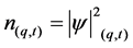with velocity, obeying to the equations [8]

, (1)

, (2)

, (3)

where

, (4)

where

(5)

is the Hamiltonian of the system and where is the quantum pseudo-potential that reads

. (6)

Equations (1)-(3) with the identity

(7)

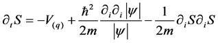
can be derived [33] [34] by the system of two coupled differential equations

(8)

(9)

by taking the gradient of (8) and multiplying Equation (9) by. It is straightforward to see that the system of equations (8)-(9) for the complex variable

(11)

is equivalent to equate to zero the real and imaginary part of the Schrödinger equation

. (12)

The stochastic generalization can be established by consider the presence of a noise as a function of both time and space.

For the sufficiently general case, to be of practical interest, can be assumed Gaussian with null correlation time, the space is assumed isotropic and the noises on different co-ordinates independent. Thence, the stochastic partial differential conservation equation for reads [32]

(13)

(14)

, (15)

, (16)

(17)

where T is the noise amplitude parameter (e.g., the temperature of an ideal gas thermostat in equilibrium with the system [32] ) and is the dimensionless shape of the spatial correlation function of.

The condition that the energy fluctuations due to the quantum potential do not diverge, as T goes to zero (so that the deterministic limit (i.e., the quantum mechanics) can be warranted) leads to a owing the form [32]

. (18)

The noise spatial correlation function (18), is a direct consequence of the derivatives present into the quantum potential that give rise to an elastic-like contribution to the system energy that reads [34]

, (19)

where a large “curvature” of leads to high quantum potential energy.

This can be easily checked by calculating the quantum potential of the wave function that reads

(20)

showing that the energy increases as the inverse squared of the distance between two adjacent peaks (i.e., the wave length). In the stochastic case, these peaks can be generated by two independent fluctuations of the wave function modulus where represents (as a mean) the correlation distance of such fluctuations.

Therefore, particle density independent fluctuations very close each other (i.e.,), generating very high curvature on the density, can lead to a whatever large quantum potential energy even in the case of vanishing fluctuations amplitude (i.e.,).

In this case the convergence of Equations (13-17) to the deterministic limit (1)-(3) (i.e., the standard quantum mechanics) would not happen. Therefore, in order to eliminating these unphysical solutions, the additional conditions (22) comes into the set of the quantum equations [32] in order to rule out unphysical solutions.

If we require that (following the criterion that higher is the energy lower is the probability to reach the corresponding (i.e., state with infinite energy have zero probability to realize itself) it follows that independent fluctuations of the density on shorter and shorter distance are progressively suppressed (i.e., have lower and lower probability of happening). This physical effect due to the quantum potential (that confers to the particle density function the elastic behavior like a membrane, very rigid against short range curvature) imposes a finite correlation length to the possible physical fluctuations.

In the small noise limit [32] the suppression of particle density fluctuations on very short distance, due to the finite energy requirement, brings to a restriction on the correlation length of the noise itself [32] that reads

, (21.a)

and to the expression for that reads

(21.b)

leading to explicit form of the variance (18)

(21.c)

where is a constant with the dimension of a migration coefficient.

Furthermore, the action (17), that can be re-cast in the form [32]

, (22)

in the case of very small noise amplitude (close to the deterministic quantum mechanical limit) due to the constraints (21.c), owns a that is a small fluctuating quantity [32] .

Finally, it is worth mentioning that for T > 0 the stochastic Equations (13)-(17) can be obtained by the following system of differential equations

(23)

(24)

which for the complex wave function are equivalent to following the stochastic version of the Schrödinger equation [33]

. (25)

3. Quantization of motion in the Hydrodynamic Model

In order to establish the hydrodynamic analogy, the gradient of action has to be considered as the momentum of the particle. When we do that, we broaden the solutions so that not all momenta solutions of the hydrodynamic equations can be solutions of the Schrödinger problem.

As well described in Ref. [12] , the state of a particle in the QHEs is defined by the real functions and.

The restriction of the solutions of the QHEs to those ones of the standard quantum problem comes from additional conditions that must be imposed in order to warrant the existence of the action function by the field of the particle momenta.

The integrability of the action gradient, in order to have the scalar action function S, is warranted if the probability fluid is irrotational, that being

(26)

is warranted by the condition

(27)

so that it holds

(28)

Moreover, since the action is contained in the exponential argument of the wave function, all the multiples of, with

(29)

are accepted.

3.1. Characteristics of eigenstates

Below, we will show how the problem of finding the quantum eigenstates can be carried out in the hydrodynamic description. Since the method does not change either in classic approach or in the relativistic one, we give here an example in the simple classical case of a classical harmonic oscillator.

In the hydrodynamic description, the eigenstates are identified by their property of stationarity that is given by the “equilibrium” condition

(30)

(that happens when the force generated by the quantum potential exactly counterbalances that one stemming from the Hamiltonian potential) with the initial “stationary” condition

. (31)

The initial condition (31) united to the equilibrium condition leads to the stationarity along all times and, therefore, by (30) the eigenstates are irrotational.

Since the quantum potential changes itself with the state of the system, more than one stationary state (each one with its own) is possible and more than one quantized eigenvalues of the energy may exist.

For a time independent Hamiltonian, whose hydrodynamic energy reads [34] , with eigenstates (for which it holds) it follows that

(32)

and that that represents the differential equation, that in the quantum hydrodynamic description,

allows to derive to the eigenstates. For instance, for a harmonic oscillator (i.e.,) such differential equation reads

. (33)

If for (33) we search a solution of type

, (34.a)

we obtain that and (where represents the n-th Hermite polynomial). Therefore, the generic n-th eigenstate reads

. (34.b)

From (34.b) it follows that the quantum potential of the n-th eigenstate reads

(35)

where it has been used the recurrence formula of the Hermite polynomials, that by (33) leads to

(36)

The same result comes by the calculation of the eigenvalues that read

(37)

where and where. Moreover, by using (32), (36)-(37) for eigenstates it follows that

, (38.a)

. (38.b)

Confirming the stationary equilibrium condition of the eigenstates.

Finally, it must be noted that since all the quantum states are given by the generic linear superposition of the eigenstates (owing the irrotational momentum field) it follows that all quantum states are irrotational. Moreover, since the Schrödinger description is complete, do not exist others quantum irrotational states in the hydrodynamic description.

3.2. The Quantization of the Stochastic hydrodynamic motion Equations

In the QHA, the non-locality does not come from boundary conditions (that are apart from the equations) but from the quantum pseudo-potential (6) that depends by the state of the system and is a source of an elastic-like energy [8] [32] [34] .

If we consider a bi-dimensional space, the quantum potential makes the vacuum acting like an elastic membrane that becomes quite rigid against curvature (i.e., fluctuations) on very small distances.

Given that the force of the quantum potential in a point depends by the state of the system around it, it introduces the non-local character into the motion equations.

Being so, the quantum non-local properties can be very well identified and studied by means of the analytical mathematical investigations of the property of the quantum potential (6).

This fact is even more important in presence of fluctuations since the quantum potential, containing the second partial derivatives of the wave function modulus, is critically dependent by the distance on which independent fluctuations happen.

The derivation of the correlation length of the noise from the condition of non-diverging energy of the quantum potential short-distance fluctuations brings a quite heavy stochastic calculation and is out of the purpose of this paper [32] .

Nevertheless, from the general point of view, we can observe that if goes to infinity respect to the physical length of the system (i.e., microscopic mass or low temperature) the noise variance (14) becomes a pure function of time and reads

. (39)

Moreover, given the dependence of the amplitude of noise variance, it goes to zero (as well as in (22)) and the deterministic standard quantum equations are recovered in the limit [32] .

In this case, the ensemble of forbidden values for the action due to the quantization constraint (deterministic limit) reaches the well-known characteristic of the quantum mechanics form.

On the contrary, when fluctuations are present, the stochastic quantum hydrodynamic analogy leads to a scenario where the domain of forbidden states becomes smaller and smaller as the fluctuations amplitude increases (see figure 1).

In order explain the phenomenon depicted in figure 1, we observe that the quantum force cannot be taken out by the deterministic PDE (1) [8] [34] because this operation will wipe out the eigenstates deeply changing the structure of such equation.

The presence of the QP is needed for the realization of the quantum stationary states (i.e., eigenstates) that happen when the force of the QP exactly balances the Hamiltonian one.

On the other hand, when we deal with large-scale systems with physical length and when fluctuations are present in weakly interacting systems, we can have a vanishing small quantum force at large distances (see Appendix A) [17] [31] [32] that, being much smaller than fluctuations, becomes ineffective to the evolution

of the system (and can be neglected in the motion equations). In this case, not only the action can take whatever value but the quantization itself is physically lost.

It must be underlined that not all types of interactions lead to a vanishing small quantum force at large distance (a straightforward example is given by linear systems where the quantum potential owns a quadratic form (see appendix A) [17] [32] .

Nevertheless, it exists a large number of non-linear long-range weak potentials (e.g., Lennard Jones types) where the quantum potential tends to zero (see Appendix A) at infinity and can be neglected [31] . In this case, a rarefied gas of such interacting particles behaves as a classical phase when the mean particle distance is much larger that the quantum potential range of interaction [17] [31] [32] .

In the following we analyze the large scale form of the SPDE (13) both for finite and infinite quantum potential range of interaction.

In order to investigate this point, let’s consider a system whose Hamiltonian reads

, (40)

in this case the equations (1)-(3) can be derived by the following phase-space equation

(41)

where

. (42)

(43)

(44)

by integrating equation (41) over the momentum p with the conditions that with the constraint on the quantum phase space density

. (45)

The factor (namely the wave-particle equivalence) warrants the correspondence rule

(46)

between the quantum hydrodynamic model and the Schrödinger equation [8] [33] [34] .

When a spatially distributed random noise is present, the phase SPDE, whose zero noise limit is the deterministic PDE (41), reads

. (47)

Near the deterministic limit, in the case of Gaussian noise (8), it is possible to re-cast (47) as

, (48)

where in is the solution of the PDE (1) and where, where

(49)

where.

Thanks to conditions (21.a-21.b) [32] , closer and closer we get to the deterministic limit (i.e.,) , smaller and smaller is the amplitude of the random term on the right side of (48)

(50)

When the standard quantum mechanics is achieved and the quantum potential cannot be disregarded from the hydrodynamic quantum motion equations.

On the contrary, when, in weakly bounded system when the force steaming from the quantum potential at large distance tends to zero (and becomes much smaller than its fluctuations) it is possible to coherently define [32] a measure of the quantum potential range of interaction that reads [32]

. (51)

Thence, when it follows that

(52)

where formula (52) expresses the fact that the quantum potential force is much smaller than its fluctuations and, hence, that

. (53)

For sake of completeness, we observe that close to the deterministic limit (i.e., to the quantum mechanics) when the quantum potential cannot be disregarded even if it is vanishing small, therefore the quantum potential range of interaction is physically meaningful if and only if. For the quantum potential range of interaction must be retained equal to.

Introducing (53) into Equation (48) it follows that

(54)

Equation (54) for small but not null noise amplitude T (i.e., for and m equal to the proton mass, where is defined by setting) leads to the stochastic phase space PDE

(55)

where is a small random quantity, that shows dynamics that fluctuate around a deterministic “classical” core and that do not own eigenstates.

Physically speaking, the central point in weakly quantum entangled systems, whose characteristic length is much bigger than the quantum potential range of interaction, is that the stochastic sequence of fluctuations of the quantum potential does not allow the coherent reconstruction of the superposition of state since they are much bigger than the quantum potential itself. In this case (especially in classically chaotic systems) the effect of the quantum potential with fluctuations (even with null time mean) on the dynamics of the system is not equal to the effect of its average.

If the quantum potential can be disregarded in a large scale description, the action (22) reads

(56)

and hence, the momentum of the solutions given by the δ-function in (45) (i.e., approaches the classical value (plus a small fluctuation) and reads

(57)

When we deal with a huge scale system (i.e.,) given the macroscopic scale, the quantized action values become very dense and the allowed action ones fill all the space (see figure 1). Moreover, in weakly interacting systems we may actually have that quantization is ineffective.

Observing that the quantum coherence length results by the geometrical mean of the stochastic length

(of order of unity or less, about (1.44 cm at 1˚K)) and the Compton length (the reference length

for the standard quantum mechanics) it follows that the description of a macroscopic system (with a resolution such as) is classically stochastic at laboratory scale, even at low temperature, since for as small as the temperature of the background radiation 2725˚K, it results

for a particle of proton mass (or at a temperature of 300˚K)). Even if the condition is usually satisfied for macroscopic objects constituted by Lennard-Jones interacting particles, there also exists (at laboratory condition) the possibility to have and, hence, to detect quantum phenomena. The most direct and immediate way is to consider observables depending by molecular properties of solid crystals that, due to the linearity of the particles interaction, can own a very large quantum potential range of action (that may result of order of ten times of the atomic distances [17] ). Another possibility is to refrigerate a fluid below the critical density (if it does not undergo solidification) in order to obtain that the mean molecular distance becomes smaller than or [31] .

4. Discussion

Non-linear systems of particles weakly-interacting, to which equation (54) can apply, are wide-spread in nature.

For instance, Equation (54) can apply to a rarefied gas phase particles interacting by a Lennard-Jones type potential where the mean inter-particle distance is much bigger than and (for instance for the helium at room temperature it results [31] ). In this case, the quantum superposition of states of molecules (or group of them) do not exist and the gas system behaves classically.

A deeper analysis [17] , shows that the classical behavior of molecules of a real gas is maintained down to the density of liquids. On the contrary, due to the linearity of intermolecular forces in crystals, becomes bigger than the mean inter-particle distance [17] and the quantum behavior of groups of atoms is maintained. Nevertheless, since the linear interaction of solids ends over a certain distance, the quantum behavior survives just in phenomena at the molecular scale (e.g., Braggs diffraction).

From this output, the stochastic quantum hydrodynamic model gives a realistic answer to the Schrödinger’s cat enigma: such a cat (made of ordinary weakly interacting molecules) cannot have a macroscopic dimension in a noisy environment.

Furthermore, it is worth mentioning that in the classical macroscopic reality when we try to detect microscopic variables, below a certain limit, the wave dual properties of particles emerge.

If in the classical macroscopic reality the position and velocity are perceived independent, on microscopic scale the wave-particle property (e.g., the impossibility to interact just with a part of a system without perturbing it entirely) leads to the coupling between conjugated variables such as position and velocity.

The scale-dependence of the quantum potential interaction leads the classical perception of the reality until the resolution is at least larger than the quantum coherence length.

Moreover, we observe that higher is the amplitude of the noise t, smaller is the length and, hence, higher is the attainable degree of spatial precision within the classical scale.

On the other hand, higher is the amplitude of noise, larger is the variance of energy measurements and/or related quantity such as the velocity.

It is straightforward to show that this mutual effect on conjugated variables in presence of noise obeys to the Heisenberg’s principle of uncertainty.

In fact, by using the quantum stochastic hydrodynamic model, it is possible to derive the uncertainty relation between the time interval of a measurement and the related variance of the energy on a particle of mass m.

If on distances smaller than any system owns quantum properties, like a wave, any its subparts cannot be perturbed without disturbing all the entire system, it follows that the independence between the measuring apparatus and the measured system (classical freedom) requires that they must be far apart, at least, more than

and, hence, for the finite speed of propagation of interactions and information (local relativistic causality (LRC)) the measure process must last longer than the time.

Moreover, given that the noise in (13) can generally be very small, the energy fluctuations are Gaussian [32] and the mean value of the energy fluctuations per degree of freedom is [35] and thence, in the non-relativistic limit () for a particle of mass m, the energy variance reads

(58)

from which it follows that [32] [35]

. (59)

It is worth noting that the product is constant since the growing of the energy variance

with the square root of the temperature is exactly compensated by the decrease of the mini-

mum time of measurement

(60)

furnishing an elegant physical explanation why the Eisenberg relations exist in term of a physical constant.

The same result is achieved if we derive the uncertainty relation between the position and the momentum of a particle of mass m.

If we measure the spatial position of a particle with a precision of so that we do not perturb its

quantum wave function (spontaneously localized on a spatial domain of order of) the variance of the modulus of its momentum due to the vacuum noise reads

(61)

leading to the uncertainty relation

(62)

If we impose of measuring the spatial position with a higher precision (i.e.,), we have to localize the quantum state of the particle more than what spontaneously is.

Due to the increase of spatial confinement of the wave function, the increase of the quantum potential energy (due to the increase of curvature of n) as well as of its variance are generated. As a consequence of this, the particle momentum variance increases too.

Since the correlation between the wave-function localization and momentum variance are submitted to the properties of the Fourier transform relations (holding for any wave) the uncertainty relations remain satisfied if we try to localize the wave function either by environmental fluctuations or by physical means (i.e., external potentials)).

In the frame of the stochastic QHA (SQHA) the achievement of the classical mechanics is achieved as a scale-mediated effect.

The SQHA shows that the classical freedom principle (independence between systems), the local relativistic causality can be achieved and made compatible with the quantum mechanics, and the uncertainty principle, in the frame of a unique theory [35] .

The possibility of classical freedom derives from the fact that weakly bounded systems can disentangle themselves beyond the quantum coherence lengths and.

Moreover, it is noteworthy to note that the quantum mechanics recovered as the deterministic limit of a stochastic theory, fulfills the philosophical need of determinism [1] - [3] . In the SQHA model the quantum mechanics represent the deterministic limit of a stochastic theory. In this picture, the quantum distributions are deterministic and well defined once the initial distributions and boundary conditions are defined. Under this light the hydrodynamic model gives its answer to the God-enigma: God does not play dice.

Moreover, in the SQHA, the wave-function collapse to an eigenstate (due to an interaction (i.e., measurement) in a classical fluctuating environment) is not described with the help of statistical measurements (out of the theory) but can be described by the theory itself as a kinetic process to a stationary state. This fact leads to a quantum theory with the conceptual property of a complete theory.

From experimental point of view, in order to demonstrate that the local relativistic causality (LRC) breaks down in quantum processes, it needs to demonstrated that the time of measurement (not smaller than the wave function decoherence time) is so short that the wave function collapse to the eigenstate is faster than the light to travel the distance over which the quantum entangled state is localized (i.e., and). Therefore, it is sufficient to demonstrate that

but, since the environmental energy fluctuations for the particle are given by (21.a), it follows that, the SQHA model shows that the LRC breaking is equivalent to prove the violation of the Heisenberg’s uncertainty principle.

From the theoretical point of view the satisfaction of the Lorentz invariance of the relativistic hydrodynamic quantum model enforce the hypothesis of compatibility between the LRC and the quantum nonlocality.

Given that the invariance of light speed is the generating property of the Lorentz transformations, the co-var- iant form (i.e., invariant 4-scalar product) of quantum potential [36]

(63)

united to the property of the spacetime wave function that changes accordingly with the Lorentz transformation, allows affirming that the quantum non-local behavior (deriving by the quantum potential) is compatible with the postulate of the relativity of the maximum speed of propagation of interactions.

In fact, whatever inertial system we choose moving with velocity v < c, the quantum potential (63) realizes the quantum dynamics in such new reference system (where the light speed is always c and hence not attainable). This fact forbids that in any inertial system the time difference between the initial conditions (e.g., starting of measurement (i.e., cause)) and the final one (wave collapse (i.e., effect)) is null so that the quantum-potential action on the whole wave function (sometime de-localized on very far away points) cannot realize itself in a null time (or it can known before it happens).

The compatibility between the quantum mechanics and the postulate of light speed invariance of the relativity can find its full demonstration inside a theory able to describe the kinetic of the wave function collapse during the measurement process.

Actually, the formulation of the standard quantum theory, based on statistical postulates concerning the measurement process, makes it a semi empirical theory unable to describe the “quantum irreversible” processes (such as the measurement one) while a closed (self-standing) quantum theory must be able to describe the measuring process itself.

To this end the SQHA shows to be a good candidate for describing the quantum behavior in presence of noise allowing the description of the quantum decoherence and the quantum to classical transition [12] [22] - [36] .

5. Conclusions

In the present paper, the effect of the spatially distributed stochastic noise on quantum mechanics is analyzed.

The work shows how the quantum potential generates the non-local quantum behavior (eigenstates and coherent superposition of states) and the multiple quantized action values.

The analysis shows that in the quantum stochastic hydrodynamic model it is possible to maintain the concept of freedom of the classical reality between systems far apart beyond the range of interaction of quantum potential as well as to make compatible the local relativistic causality with the uncertainty principle.

In the SQHA, the collapse of the wave-function due to the interaction with a classical object (in presence of environmental fluctuations) can be described inside the model itself so that it can be assimilated to a relaxation process to a stationary state (eigenstate).

The SQHA allows showing that the conditions on the measurement duration time are compatible with the relativistic postulate of invariance of light speed and the quantum uncertainty principle.

The paper shows that this hypothesis has the theoretical support of the Lorentz invariance of the relativistic quantum potential that generates the nonlocal behavior of the quantum mechanics.

Cite this paper

Piero Chiarelli, (2016) Quantum Decoherence Induced by Fluctuations. Open Access Library Journal,03,1-20. doi: 10.4236/oalib.1102466

References

Appendix A

A.1. Quantum Interaction on Large distance

The large-distance limit of the quantum force allow us to obtain the macro-scale form of equations (42)-(47). For sake of simplicity, we discuss the one-dimensional case with that at large distance goes like

(A.1)

where is a polynomial of degree equal to k, is the macroscopic variable (where,

where is the macro-scale resolution) and is the range of the QP interaction. By using (A.1), the QP (6) at large scale reads

(A.2)

where.

Thence, for (i.e.,) finite, the quantum force at large scale (i.e., ,) reads

(A.3)

Moreover, since the integral

(A.4)

converges for, (A.4) tells us if the QP force is negligible on large scale as given by (A.3). Therefore, finite values of the mean weighted distance

, (A.5)

warrants the vanishing of QP at large distance and, hence, it can be assumed as an evaluation of the quantum potential range of interaction.

It is worth mentioning that condition (A.4) is not satisfied by linear systems whose eigenstates have [24] , so that and they cannot admit the classical limit.

It is also worth noting that condition (A.4), obtained for (WFM) owing the form (A.1), also holds in the case of oscillating wave functions whose modulus is of type

(A.6)

where are polynomials of degree equal to p. In this case, in addition to the requisite, the conditions and are required to warrant (A.4) [32] .

For instance, the Lennard-Jones-type potentials holds and, hence, they own finite.

In the multidimensional case, depends by the path of integration and (A.5) reads

(A.7)

where and is the incremental vector tangent to.

Since, the physical meaning of must be independent by the path of integration (we know that is

integrable but we do not know nothing about the integrability of) in order to well define, the

fixation of the integral path is needed. If we choose the integration path where is a generic versor, reads

(A.8)

Moreover, since in order to evaluate at what distance the quantum force becomes negligible whatever is the direction of the versor, among the values of (A.8) we must consider the maximum one so, finally, reads

(A.9)

A.2. Strength of quantum Coherence

In order to evaluate the quantum coherence strength we analyze the quantum potential characteristics at large distance.

Fixed the WFM at the initial time, then the Hamiltonian potential and the quantum one determine the evolution of the WFM in the following instants that on its turn modifies the quantum potential.

A Gaussian WFM has a parabolic repulsive quantum potential, if the Hamiltonian potential is parabolic too (the free case is included), when the WFM wideness adjusts itself to produce a quantum potential that exactly compensates the force of the Hamiltonian one, the Gaussian states becomes stationary (eigenstates). In the free case, the stationary state is the flat Gaussian (with an infinite variance) so that any free Gaussian WFM expands itself following the ballistic dynamics of quantum mechanics since the Hamiltonian potential is null and the quantum one is a quadratic repulsive one.

From the general point of view, we can say that if the Hamiltonian potential grows faster than a harmonic one, the wave equation of a self-state is more localized than a Gaussian one and this leads to a stronger-than a quadratic quantum potential.

On the contrary, a Hamiltonian potential that grows slower than a harmonic one will produce a less localized WFM that decreases slower than the Gaussian one, so that the quantum potential is weaker than the quadratic one and it may lead to a finite quantum non-locality length (A.5).

More precisely, as shown above, the large distances exponential-decay of the WFM given by (A.1) with k < 3/2 is a sufficient condition to have a finite quantum non-locality length [17] .

In absence of noise, we can enucleate three typologies of quantum potential interactions (in the unidimensional case):

1) k > 2 strong quantum potential that leads to quantum force that grows faster than linearly and is infinite (super-ballistic expansion for the free particle WFM) and reads

(A.10)

2) k = 2 that leads to quantum force that grows linearly

(A.11)

and is infinite (ballistic expansion for the free particle WFM).

3) “middle quantum potential”; the integrand of (A.4) will result

. (A.12)

e quantum force remains finite or even becomes vanishing at large distance but may be still infinite (under- ballistic expansion for the free particle WFM).

4) k < 3/2 “week quantum potential” interaction leading to quantum force that becomes vanishing at large distance following the asymptotic behavior

(A.13)

with a finite for (asymptotically vanishing expansion for the free particle WFM).

A.3. Pseudo-Gaussian particle

Gaussian particles generate a quadratic quantum potential that is not vanishing at large distance and hence cannot lead to classical dynamics. Nevertheless, imperceptible deviation by the perfect Gaussian WFM may possibly lead to finite quantum non-locality length. Particles that are inappreciably less localized than the Gaussian ones

(let’s name them as pseudo-Gaussian) own that can sensibly deviate by the linearity so that the quantum non-locality length may be finite.

We have seen above that for k < 3/2 (when the WFM decreases slower than a Gaussian) a finite range of interaction of the quantum potential is possible.

The Gaussian shape is a physically good description of particle localization, but irrelevant deviations from it, at large distance, are decisive to determine the quantum non-locality length.

For instance, let’s consider the pseudo-Gaussian wave-function type

(A.14)

where is an opportune regular function obeying to the condition

(A.15)

For small distance it holds

(A.16)

and the localization given by the WFM is physically indistinguishable from a Gaussian one, while for large distance we obtain the behavior

. (A.17)

For instance, we may consider the following examples

a)

(A.18)

; (A.19)

b)

(A.20)

; (A.21)

c)

(A.22)

; (A.23)

d)

(A.24)

(A.25)

All cases a)-d) lead to a finite quantum non-locality length.

In the case d) the quantum potential for reads

(A.26)

leading, for 0 < k < 2, to the quantum force

(A.27)

that for k < 3/2 gives,

It is interesting to note that for k =2 (linear case)

(A.28)

the quantum potential is quadratic

, (A.29)

and the quantum force is linear (repulsive) and reads

(A.30)

The linear form of the force exerted by the quantum potential leads to the ballistic expansion (variance that grows linearly with time) of the free Gaussian quantum states.

References

- 1. Bell, J.S. (1964) On the Einstain-Podolsky-Rosen Paradox. Physics, 1, 195-200.
- 2. Einstein, A., Podolsky, B. and Rosen, N. (1935) Can Quantum-Mechanical Description of Physical Reality Be Considered Complete? Physical Review, 47, 777-780.
http://dx.doi.org/10.1103/PhysRev.47.777 - 3. Greenberger, D.M., Horne, M.A., Shimony, A. and Zeilinger, A. (1990) Bell’s Theorem without Inequalities. American Journal of Physics, 58, 1131-1143.
http://dx.doi.org/10.1119/1.16243 - 4. Bialyniki-Birula, I., Cieplak, M. and Kaminski, J. (1992) Theory of Quanta. Oxford University Press, New York Oxford, 278.
- 5. Bohm, D. (1952) A Suggested Interpretation of the Quantum Theory in Terms of “Hidden” Variables. I. Physical Review, 85, 166.
http://dx.doi.org/10.1103/PhysRev.85.166 - 6. Madelung, E. (1927) Quantentheorie in Hydrodynamischer Form. Zeitschrift für Physik, 40, 322-326.
http://dx.doi.org/10.1007/BF01400372 - 7. Jánossy, L. (1962) Zum hydrodynamischen Modell der Quantenmechanik. Zeitschrift für Physik, 169, 79-89.
http://dx.doi.org/10.1007/BF01378286 - 8. Bialyniki-Birula, I., Cieplak, M. and Kaminski, J. (1992) Theory of Quanta. Oxford University Press, New York Oxford, 87-111.
- 9. Nelson, E. (1966) Derivation of the Schrödinger Equation from Newtonian Mechanics. Physical Review, 150, 1079.
http://dx.doi.org/10.1103/PhysRev.150.1079 - 10. Nelson, E. (1967) Dynamical Theory of Brownian Motion. Princeton University Press, London.
- 11. Nelson, E. (1985) Quantum Fluctuations. Princeton University Press, New York.
- 12. Guerra, F. and Ruggero, P. (1973) New Interpretation of the Euclidean-Markov Field in the Framework of Physical Minkowski Space-Time. Physical Review Letters, 31, 1022.
http://dx.doi.org/10.1103/PhysRevLett.31.1022 - 13. Parisi, G. and Wu, Y.-S. (1981) Perturbation Theory without Gauge Fixing. Scientia Sinica, 24, 483.
- 14. Jona, G., Martinelli, F. and Scoppola, E. (1981) New Approach to the Semiclassical Limit of Quantum Mechanics. Communications in Mathematical Physics, 80, 233-254.
- 15. Ruggiero, P. and Zannetti, M. (1982) Stochastic Description of the Quantum Thermal Mixture. Physical Review Letters, 48, 963.
http://dx.doi.org/10.1103/PhysRevLett.48.963 - 16. Ruggiero, P. and Zannetti, M. (1983) Microscopic Derivation of the Stochastic Process for the Quantum Brownian Oscillator. Physical Review A, 28, 987.
http://dx.doi.org/10.1103/PhysRevA.28.987 - 17. Chiarelli, P. (2013) Quantum to Classical Transition in the Stochastic Hydrodynamic Analogy: The Explanation of the Lindemann Relation and the Analogies between the Maximum of Density at Lambda Point and That at the Water-Ice Phase Transition. Physical Review & Research International, 3, 348-366.
- 18. Weiner, J.H. and Askar, A. (1971) Particle Method for the Numerical Solution of the Time-Dependent Schrödinger Equation. The Journal of Chemical Physics, 54, 3534.
http://dx.doi.org/10.1063/1.1675377 - 19. Weiner, J.H. and Forman, R. (1974) Rate Theory for Solids. V. Quantum Brownian-Motion Model. Physical Review B, 10, 325.
http://dx.doi.org/10.1103/PhysRevB.10.325 - 20. Terlecki, G., Grun, N. and Scheid, W. (1982) Solution of the Time-Dependent Schrödinger Equation with a Trajectory Method and Application to H+-H Scattering. Physics Letters A, 88, 33-36.
http://dx.doi.org/10.1016/0375-9601(82)90417-0 - 21. Gardner, C.L. (1994) The Quantum Hydrodynamic Model for Semiconductor Devices. SIAM Journal on Applied Mathematics, 54, 409-427.
http://dx.doi.org/10.1137/S0036139992240425 - 22. Bret, J.D., Gupta, S. and Zaks, A. (1984) Stochastic Quantization and Regularization. Nuclear Physics B, 233, 61-87.
http://dx.doi.org/10.1016/0550-3213(84)90170-6 - 23. Zwanziger, D. (1984) Covariant Quantization of Gauge Fields without Gribov Ambiguity. Nuclear Physics B, 192, 259-269.
http://dx.doi.org/10.1016/0550-3213(81)90202-9 - 24. Mariano, A., Facchi, P. and Pascazio, S. (2001) Decoherence and Fluctuations in Quantum Interference Experiments. Fortschritte der Physik, 49, 1033-1039.
- 25. Cerruti, N.R., Lakshminarayan, A., Lefebvre, T.H. and Tomsovic, S. (2000) Exploring Phase Space Localization of Chaotic Eigenstates via Parametric Variation. Physical Review E, 63, 016208.
http://dx.doi.org/10.1103/PhysRevE.63.016208 - 26. Calzetta, E. and Hu, B.L. (1995) Quantum Fluctuations, Decoherence of the Mean Field, and Structure Formation in the Early Universe. Physical Review D, 52, 6770-6788.
http://dx.doi.org/10.1103/PhysRevD.52.6770 - 27. Wang, C., Bonifacio, P., Bingham, R. and Mendonca, J.T. (2008) Detection of Quantum Decoherence Due to Spacetime Fluctuations. 37th COSPAR Scientific Assembly, Montréal, 13-20 July 2008, 3390.
- 28. Lombardo, F.C. and Villar, P.I. (2005) Decoherence Induced by Zero-Point Fluctuations in Quantum Brownian Motion. Physics Letters A, 336, 16-24.
http://dx.doi.org/10.1016/j.physleta.2004.12.065 - 29. Bousquet, D., Hughes, K.H., Micha, D.A. and Burghardt, I. (2001) Extended Hydrodynamic Approach to Quantum-Classical Nonequilibrium Evolution. I. Theory. The Journal of Chemical Physics, 134, 064116.
http://dx.doi.org/10.1063/1.3553174 - 30. Morato, L.M. and Ugolini, S. (2011) Stochastic Description of a Bose-Einstein Condensate. Annales Henri Poincaré, 12, 1601-1612.
http://dx.doi.org/10.1007/s00023-011-0116-1 - 31. Chiarelli, P. (2014) The Quantum Potential: The Missing Interaction in the Density Maximum of He4 at the Lambda Point? American Journal of Physical Chemistry, 2, 122-131.
http://dx.doi.org/10.11648/j.ajpc.20130206.12 - 32. Chiarelli, P. (2013) Can Fluctuating Quantum States Acquire the Classical Behavior on Large Scale? Journal of Advanced Physics, 2, 139-163.
- 33. Chiarelli, P. (2013) The Classical Mechanics from the Quantum Equation. Physical Review & Research International, 3, 1-9.
- 34. Weiner, J.H. (1983) Statistical Mechanics of Elasticity. John Wiley & Sons, New York, 315-317.
- 35. Chiarelli, P. (2013) The Uncertainty Principle Derived by the Finite Transmission Speed of Light and Information. Journal of Advanced Physics, 3, 257-266.
- 36. Chiarelli, P. (2015) The Quantum Limit to the Black Hole Mass Derived by the Quantization of Einstein Equation. Class. Quantum Physics. ArXiv: 1504.07102.