Open Access Library Journal
Vol.02 No.12(2015), Article ID:69008,9 pages
10.4236/oalib.1102272
Cumulative Perturbations Affecting a Spacecraft on a Mars Equatorial Orbit from the Waxing and Waning of the Polar Caps of the Planet
Jean-Pierre Barriot
Geodesy Observatory of Tahiti, University of French Polynesia, Faa’a, Tahiti

Copyright © 2015 by author and OALib.
This work is licensed under the Creative Commons Attribution International License (CC BY).
http://creativecommons.org/licenses/by/4.0/


Received 5 December 2015; accepted 19 December 2015; published 23 December 2015
ABSTRACT
We demonstrate in this paper that periodic variations of the J2 gravity coefficient of a planet induce small cumulative perturbations on a given family of circular equatorial orbits, and that these perturbations could be measurable with current radiosciences technology. For this purpose, we first consider a Poincaré expansion of the Newtonian equations of motion. Then, by using Floquet’s theory, we demonstrate that, unlike the excitation mechanism, the perturbations are non- periodic, and that the orbit is not “stable” in the long-term, with perturbations growing exponentially. We give the full theory and an application to the case of planet Mars.
Keywords:
Mars’ Length-of-Day, Orbit Perturbations, Floquet’s Theorem
Subject Areas: Geodesy, Geophysics

1. Rationale
Chao and Rubincam [1] demonstrated that the J2 harmonic moment of Mars is subject to large annual variation as about one quarter of the CO2 atmosphere condenses during winters at the poles, and sublimes during summers (see Figure 1), with


Figure 1. The hourglass model of the sublimation/condensation mechanism on Mars. No terrestrial phenomenon is known to produce a mass redistribution of such a magnitude over a year.
where ;
;  is an arbitrary phase; s is the annual length-of-day variation; C0 is the Mars
mean polar inertial moment; Ω0 is the mean Mars angular rotation velocity; ω is the mean Mars angular orbital velocity; R is the Mars radius; and M is the planet’s mass. Similar variations, but of a lesser amplitude, are also observed on the Earth. In this paper, we show that these small variations can end up in cumulative perturbations on selected families of orbits. This work can be easily extended to semi-annual perturbations and larger degree and order gravity coefficients [2] . The only restriction is that these perturbations must have commensurate periods.
2. Orbital Mechanics
With respect to a given inertial cartesian coordinate frame, the Newtonian equations of motion of a space probe orbiting a planet are
where ,
,  is the gravitational constant of Mars,
  ,
,  represents the re-
maining part of the gravity field (without the J2 term), and the  term summarizes all the other forces like atmospheric drag (the main contributor for low orbits), sun tidal acceleration, solar pressure, relativistic corrections, etc. We use the notation
 , where
  is a global scaling factor [3] , to emphasize the fact that these forces are of small amplitudes with respect to the central and J2 terms. The aims of the notation
  is similar.
We now consider a probe orbiting the planet on a high altitude (i.e. with ) near equatorial orbit (i.e. with
 ) in order to avoid the atmospheric drag (i.e. with
 ). Up to the first order in z, this leads to
 (1)
(1)
where ,
, .
.
It is clear that the last equation is decoupled from the first two ones. The solution of the third one corresponds to an oscillation with respect to the mean orbital plane, of no interest for the following discussion.
If we switch to cylindrical coordinates , where
  and
and , we obtain
 (1’)
(1’)
The constant h0 can be identified as an angular momentum.
Jezewski [4] [5] demonstrated that if , i.e. if
 , then Equation (1’) admits a solution in terms of ellipsoidal functions as

where , and
, and  is the Jacobi ellipsoidal sine function. The two constants b and c are determined by the initial conditions, and have a direct physical meaning as the inverses
  of the periapsis and apoapsis
  of the orbit. The other two constants are given by
  and tc. One can demonstrate that
 , with
 . The constant
  is the modulus of the Jacobian sn function, and
 ,
, . The functions u and
 , viewed as a function of t are periodic, but with differ-
ent periods, and define an “ellipsis” with an apse line slowly rotating in the equatorial plane, with a period  (complete elliptic integral of the first kind). A close value of the angular velocity of the apse line can be deduced from the usual Laplace equations by summing the
  secular drifts
  of the line of node and of the line of apsides
  for a non equatorial orbit of inclination i and semi-major axis a as
 and
and ,
,  being a continuous quantity when
 , with limit
 .
.
The Hamiltonian of the unperturbed motion is given by
 (2)
(2)
If , Poincaré’s theorem [6] asserts that the equations of motion can be developed with
  as
as
 (3)
(3)
where  satisfy differential equations with null initial conditions. These differential equations are determined by plugging Equation (3) into Equation (1’), and equating the powers of
 .
.
For the first order, after some uninteresting algebra, we arrive at
 (4)
(4)
 ,
,  ,
, 
 ,
,  ,
, 
This system can be rewritten as a first order system by using the usual trick ,
, . This gives
 (5)
(5)
 , with
 .
.
Similar equations can be obtained from the formalisms of Hill or Lagrange. The approach that we retained is the simplest one. Considering an equatorial circular orbit is a fundamental assumption, as it allows us to write a very simple analytical solution.
3. Floquet’s Theory
System (5) is of Floquet’s type [7] , i.e. the coefficient matrix N is periodic, here with a period of half an orbit. More precisely, system (5) is a two-dimensional generalization of the Mathieu’s equation [8] .
The solution of the system with the second member w is given, as , by
, by
 (6)
(6)
where  is the solution of the homogeneous matrix system
 (7)
(7)
with  being the identity matrix. Because of uniqueness properties, we have
  , and therefore
 . As N is periodic with period T, i.e.
 , Floquet’s theorem asserts that the solutions
  are pseudo-periodic, i.e. that they can be written as
 , where
  is periodic with
 , and
, and  is a constant characteristic of the system, with
 . The boundedness of the solutions of systems (5) and (7) is governed by the constant matrix
 , more precisely by its spectral radius
  (the largest eigenvalue [9] ). In particular, if
 , the solution of the homogeneous system (7) is unbounded, as well as the solution of the inhomogeneous system, unless ad’hoc (and unphysical) initial conditions are imposed [10] .
4. Long-Term Behaviour of the Orbit
If  is periodic with the same period T, one can go a little farther and it can be shown (see Appendix A) that we have the geometrical series behavior [11]
 (8)
(8)
with ,
,  ,
,  ,
,  and
and ,
, .
.
This relation shows that the behavior of this system in the “long” term is governed by , as
, as  is bounded for
 . It is clear that if
  diverges, i.e. if
 , then
  diverges too, unless
 (and then
  is periodic of period T). This does not mean that the physically perturbed motion is unbounded, but that the Poincaré’s expansion (3) will break down at some stage. Physical bounds for the motion could probably be obtained by extending the works of Mioc and Stavinschi [12] - [14] to a variable J2. To obtain a common period for N and w, we just have to slightly adjust the altitude of the spacecraft, in order to have an entire number of orbital periods during a Martian year that is then becoming the common period T.
5. Numerical Results and Conclusions
Let us consider the solution for the particular case of the planet Mars and for a circular equatorial orbit. The period T of a circular equatorial orbit of radius d is given from (1’) by 
We take the numerical values from [15] [16] .
 ,
,  (unnormalized),
  ,
,  ,
,  ,
,  ,
,  (corresponding to 477 milliarcseconds).
From these values, we derive , i.e. a 10−6 relative variation with respect to the
  term.
term.
We now consider a circular orbit well beyond the atmosphere, at an altitude of 1000.629961 km (semi-major axis 4394.829961 km), in order to have exactly 6716 orbits/Martian year, corresponding to an orbital period of 147.266 min.
This leads to  for the spectral radius
  over one Martian year, from the Jordan form of the matrix C.
For the first year, the perturbations (norm of the differences between the perturbed and unperturbed motion) range up to 172.58 m in position, most of it in the along-track direction, and 122.69 mm/s in velocity. They are measurable with state-of-the-art technology, both for laser and Doppler tracking [17] , and they are slowly building up with time (see Figure 2 and Figure 3), as the spectral radius  is larger than one and
  is non zero (we have
  and
and ). A strategy to look at these pertur- bations would be to put a LAGEOS-like satellite with laser cubes [18] in such an orbit, and to observe it during

Figure 2. Building up of the position perturbations δr over the Martian years in meters. The building up of the perturbations is not strictly periodic (with a shift of about 14 minutes/year), albeit the excitation mechanism is by itself periodic.

Figure 3. Building up of the velocity perturbations δv over the years in mm/second.
a sufficient amount of time, from other Mars satellites, or even from the Earth, if it is equipped with “active” laser receptors [19] instead of passive retroreflectors.
We believe that this phenomenon is general, and that the theory described in this paper deserves to be generalized to any type of orbit, including polar orbits dedicated to mapping. The analysis will be then complicated by the presence of the secular perturbations caused by the even zonal coefficients of the gravity field, and other long period perturbations. The effect of the perturbations that originate from the triaxiality of Mars is investigated in Appendix B. We plan also to study semiannual variations of the J2 gravity coefficient, and to understand how the excitation mechanism described in this paper acts on the orbits of Phobos and Deimos that are near circular equatorial orbits.
Acknowledgements
This research was funded by the Centre National d’Etudes Spatiales (CNES).
Cite this paper
Jean-Pierre Barriot, (2015) Cumulative Perturbations Affecting a Spacecraft on a Mars Equatorial Orbit from the Waxing and Waning of the Polar Caps of the Planet. Open Access Library Journal,02,1-9. doi: 10.4236/oalib.1102272
References
- 1. Chao, B.F. and Rubincam, D.P. (1990) Variations of Mars Gravitational Field and Rotation Due to Seasonal CO2 Exchanges. Journal of Geophysical Research, 95, 14755-14760.
http://dx.doi.org/10.1029/JB095iB09p14755 - 2. Karatekin, O., Duron, J., Rosenblatt, P., Van Hoolst, T., Dehant, V. and Barriot, J.P. (2005) Mar’s Time-Variable Gravity and Its Determination: Simulated Geodesy Experiments. Journal of Geophysical Research—Planets, 110, E06001.
http://dx.doi.org/10.1029/2004JE002378 - 3. Mioc, V. and Stavinschi, M. (2004) Stability of Satellite Orbits around Nonspherical Planets. Artificial Satellites, 39, 129-133.
- 4. Jezewski, D.J. (1983) A Noncanonical Analytic Solution to the J2 Perturbed Two-Body Problem. Celestial Mechanics, 30, 343-361.
http://dx.doi.org/10.1007/BF01375505 - 5. Jezewski, D.J. (1983) An Analytical Solution for the J2 Perturbed Equatorial Orbit. Celestial Mechanics, 30, 363-371.
http://dx.doi.org/10.1007/BF01375506 - 6. Chazy, J. (1953) Mécanique Céleste. Presses Universitaires de France, Paris.
- 7. Dieudonné, J. (1980) Calcul Infinitésimal. Hermann Ed., Paris.
- 8. Angot, A. (1972) Compléments de Mathématiques. Masson et Cie Ed., Paris.
- 9. Walter, W. (1998) Ordinary Differential Equations. Springer, New-York.
- 10. Roseau, M. (1976) Equations différentielles. Masson, Paris.
- 11. Vijayaraghavan, A. (1984) An Analytic Solution for the Orbital Perturbations of the Venus Radar Mapper Due to Gravitational Harmonics. AIAA/AAS Astrodynamics Conference, Paper AIAA-84-1995.
- 12. Mioc, V. and Stavinschi, M. (1998) Stability of Satellite Motion in the Equatorial Plane of the Rotating Earth. Proceedings of the Journées des Systèmes de Référence Spatio-Temporels, N. Capitaine Ed., 257-261.
- 13. Mioc, V. and Stavinschi, M. (2001) Effects of Mars’ Rotation on Orbiter Dynamics. Proceedings of the Journées des Systèmes de Référence Spatio-Temporels, N. Capitaine Ed, 120-125.
- 14. Mioc, V. and Stavinschi, M. (2003) Stability of Equatorial Satellite Orbits. Proceedings of the Journées des Systèmes de Référence Spatio-Temporels, N. Capitaine Ed., 255-258.
- 15. Folkner, W.M., Yoder, C.F., Yuan, D.N., Standish, E.M. and Preston, R.A. (1997) Interior Structure and Seasonal Mass Redistribution of Mars from Radio Tracking of Mars Pathfinder. Science, 278, 1749-1752.
http://dx.doi.org/10.1126/science.278.5344.1749 - 16. Lemoine, F.G., Smith, D.E., Rowlands, D.D., Zuber, M.T., Neumann, G.A., Chinn, D.S. and Pavlis, D.E. (2001) An Improved Solution of the Gravity Field of Mars (GMM-2B) from Mars Global Surveyor. Journal of Geophysical Research, 106, 23359-23376.
http://dx.doi.org/10.1029/2000JE001426 - 17. Moyer, T.D. (2000) Formulation for Observed and Computed Values of Deep Space Network Data Types for Navigation. Monograph 2, Deep Space Communications and Navigation Series, JPL Publication 00-7.
- 18. Yoder, C.F., Williams, J.G., Dickey, J.O., Schutz, B.E., Eanes, R.J. and Tapley, B.D. (1983) Secular Variation of Earth’s Gravitational Harmonic J2 Coefficient from LAGEOS and Non-Tidal Acceleration of Earth’s Rotation. Nature, 303, 757-762.
http://dx.doi.org/10.1038/303757a0 - 19. Samain, E. (2002) One Way Laser Ranging on the Solar System: TIPO. Geophysical Research Abstracts, 4, Article ID: 05808.
- 20. Hu, W. and Scheeres, D.J. (2004) Numerical Determination of Stability Regions for Orbital Motion in Uniformly Rotating Second Degree and Order Gravity Fields. Planetary and Space Science, 52, 685-692.
http://dx.doi.org/10.1016/j.pss.2004.01.003
Appendix A
We have, with , by using Floquet’s theory,

with 
Therefore,  with
with ,
,  ,
,
 , and
, and ,
, . In particular, if
 , we have
 .
.
Let us verify that this formula defines a continuous mapping of .
.
For  we have

For  we have

thus proving the continuity.
Appendix B
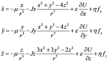
The above analysis supposes that the equatorial moments of Mars are equal. Unfortunately, because of the Tharsis uplift, Mars is the terrestrial planet for which this assumption is the least accurate. If we take into account this triaxiality, the equations of motion (1) become, in an ad’hoc reference frame and up to degree and order two [20]
 (9)
(9)
where  in the system of constants of paragraph 5 and
 . The Equations (9) can be then developed in Poincaré’s series (see Eq-
uation (3)), with respect to both  and
and . Up to the second order, and remembering that
 , we obtain
 ,
,  , and
, and . This show that the excitation mechanism described in this paper is superimposed on the motion described by Equation (9) with
  and
and  up to degree one in
  and degree two in
 . To be complete, all the other harmonic coefficients of the gravity field could be treated in the same way, provided that the circular equilibrium orbit is computed with respect to all even zonal coefficients.