Journal of Applied Mathematics and Physics
Vol.04 No.07(2016), Article ID:68908,9 pages
10.4236/jamp.2016.47132
Spectral Element Simulation of Rotating Particle in Viscous Flow
Don Liu1*, Ning Zhang2
1Department of Mathematics & Statistics, and Mechanical Engineering, Louisiana Tech University, Ruston, LA, USA
2Department of Chemical, Civil, and Mechanical Engineering, McNeese State University, Lake Charles, LA, USA


Received 29 March 2016; accepted 12 July 2016; published 15 July 2016

ABSTRACT
Spectral element methods (SEM) are superior to general finite element methods (FEM) in achieving high order accuracy through p-type refinement. Owing to orthogonal polynomials in both expansion and test functions, the discretization errors in SEM could be reduced exponentially to machine zero so that the spectral convergence rate can be achieved. Inherited the advantage of FEM, SEM can enhance resolution via both h-type and p-type mesh-refinement. A penalty method was utilized to compute force fields in particulate flows involving freely moving rigid particles. Results were analyzed and comparisons were made; therefore, this penalty-implemented SEM was proven to be a viable method for two-phase flow problems.
Keywords:
Spectral Element Method, High Order Method, Orthogonal Polynomials, Particle Fluid Intereaction, Navier-Stokes Equations, Translation and Rotation

1. Introduction
Particulate flows are of special interest to engineers and scientists [1]. Most research studies are about particles of regular shapes [1], especially spheres [2]-[7]. Markauskas [8] simulated axisymmetric particles with Discrete Element Method and analyzed the discharge rate of Hopper flow in 2006. The Arbitrary Lagrangian Eulerian technique (ALE), first appeared in 1973 [9], allows prescribed or fluid-induced adaptation of the computational mesh [6] [9] [10]. If high computational cost is permitted, ALE is ideal for particulate flows with gradual motion of finite number of particles. In 2009, Apte et al. [11] presented fully resolved simulations of moving rigid arbitrary-shaped particles with Distributed Lagrangian Multiplier (DLM) fictitious domain method implemented in a finite volume formulation. Both ALE and DLM are very accurate and comparable to direct numerical simulation. However, in terms of computational cost, both are too expensive even if for a few particles and could be very slow and cumbersome in modeling numerous interacting particles. Studies on rotational particles are relatively fewer. Bush et al. [12] conducted a comprehensive survey of both theoretical and experimental results about particle motion in rotating fluids. Tanzosh and Stone [13] analyzed particle motion in a rotating fluid for small Reynolds number with the Boundary Integral Method. Hynes et al. [14] numerically studied the rotational and translational friction of fluid on a particle and examined the DeGroot-Mazur approximation. Bluemink et al. [15] experimentally investigated a freely rotating sphere in a sloid-body rotational flow. Liu and Prosperetti [16] studied a spinning sphere subject to nonslip planar boundaries with the combined immersed- boundary and finite-difference method. Lee and Ladd [17] numerically simulated a rotating suspension of particles in Stokes flow. So far, it is uncommon to see in open literature about numerical study of a rotating particle subject to force couples simulated with a high order method. This paper presents a method and implementation for fully resolving viscous dominant flow around rotating a particle with a modal version of the spectral element method via both h-type and p-type mesh refinement.
2. Mathematical Physics of Particulate Flow
2.1. Description of the Fluid
When particles and a fluid are treated as two phases, the surfaces of particles, the moving internal boundaries, are unknown to the fluid. However, if the particles and the fluid are considered as an entire system, only those confining walls are boundaries. The exchange of drag and force couple between the fluid and particles are internal to the system. This paper presents the Virtual Identity Particle (VIP), a combined Eulerian-Lagrangian model for particulate flow. The fluid velocity is a three-dimensional solenoidal vector field and satisfies the incompressible Navier-Stokes equations with added source terms describing the exchanging momenta between particles and the fluid in an Eulerian reference frame within a Cartesian coordinate system [18]-[20].
 ,
,  ,
,  , (1)
, (1)
 , (2)
, (2)
where ρ and µ are the density and dynamic viscosity of the fluid;  is the Lagrangian coordinate vector of the particle k in reference to the origin of the Eulerian coordinates; N is the total number of particles in the fluid;
  is the added source term for the interaction between this particle and the fluid. This source term contains two groups of force fields given as the following:
 , (3)
, (3)
In which,  and
and  are the vector sum of force and torque (force couple) of the particle k to the fluid;
  is a kernel function to distribute the force and torque to the flow field; σ1, σ2 are two vectors of parameters for the geometrical features of particles. Depending on the specific complexity of a particle, the kernel function could take different forms, e.g., a transcendental function for a hemisphere or tailored polynomials for a cylinder etc. Particles in this paper are spherical but the model could handle nonspherical-ellipsoidal, semisphere or circular cylindrical particles. The kernel function is essentially a probability density funtion with a conservation property. The mass of the particle k is mp and its displaced mass of water is mf. The vector of moment of inertia about its rotating axes is
 . The particle k has a translational velocity
  and an angular velocity
 . These velocities, force and torque satisfy the Lagrangian form of the constitutional equation as below:
 , (4)
, (4)
where  and
and  are zero matrices of dimension
  and
and , respectively.
2.2. Description of Particles
After solving the fluid velocity , the velocity
  of the particle k is filtered out, as below, through a triple integral over the volume (
 ) of the computatioal domain:
 . (5)
. (5)
Similarly the angular velocity is computed with the vorticy of the fluid through another triple integral as below:
 . (6)
. (6)
The displacements in both translational and rotational motion are given by the constitutional equations:
 ,
, . (7)
. (7)
2.3. Dynamics of the Motion
For resistance problems which are defined by Kim and Karrila [21] in particulate flow, the force and torque are to be determined from known motion, such as velocity  and
and  , the following penalized differential equations are solved:
 , (8)
, (8)
 , (9)
, (9)
where τ is a pseudo-time step; and are penalty parameters for the force and torque, respectively, and their magnitude is restricted by the stability condition during explicit time integrations. During each time step, the force and torque are initialized to their values in the previous time step or zero if starting from the begining. These known values of force and torque are plugged into Equation (2), then remove the convective term and replace t into τ in Equation (2) so that it becomes an unsteady Stokes equation. After solving the unsteady Stokes problem for the fluid velocity, then Equations (5) and (6) are used to compute the predicted velocity  and
and  so that they are compared with the known values
  and
and  . If the differences are large, then use the new velocity values in Equations (8) and (9) to update the force and torque. If the differences are very small, then
  and
and  are no longer changing withτ and convergence is achieved.
For mobility problems with known values for the force and torque  and
and , Equation (2) is solved for the fluid velocity
 . Then Equations (5) and (6) are evaluated for the velocities of the particle k, and Equation (7) is integrated to obtain the translational and rotational displacements for the next time instant. If the mobility problem is to be solved for the next time, then Equation (4) is used to estimate values for
  and
and . Once values of force and torque are available, this process repeats again.
For problems without any prior knowledge of motion and force, the fluid velocity at the center of the particle k can be used as the approaching velocity and theoretical laws of fluid mechanics can estimate the drag force on this particle. For low Reynolds number particulate flow, Stokes law gives a good estimate of the drag force:
 ,
, . (10)
For finite Reynolds number flow, Oseen law gives the corresponding estimate of the drag force:
 ,
, . (11)
In order to compute the vector of force couples on the particle k, one of the force dipole iteration algorithms developed by Liu [22] will be used. Here the penalized algorithm is used and details are in the next subsection.
2.4. Penalized Dipole Iteration Scheme
After solving Equation (2), the integral averaged strain rate tensor  inside this particle is evaluated:
 , (12)
here L is the characteristic length for nondimensionlization;  is the kinematic viscosity; and
  is the rate of strain tensor for the fluid velocity field. Then the Euclidean (L2) norm of
  is computed and compared with a given tolerance (e.g., Tol = 10−4). If
  is smaller than Tol then there is no need to adjust values of force couples. Otherwise, either of below penalized differential equations is solved with the second or third order Adam-Bashforth scheme. If the dominant force on the particle k is an external body force e.g. gravity, then use
 . (13)
Otherwise, if the dominant force on the particle k is drag force and flow is pressure-gradient driven, then use
 , (14)
instead, in which r is the radius of the particle. A few iterations are needed in the penalized dipole iteration scheme to reduce  to be smaller than Tol. Further details will be elaborated later sections.
3. Numerical Method Used in Implementation
The modal spectral element method (MSEM) [23] [24] was used to implement the mathematical physics model described above. Inherited the advantage of general finite element method (FEM) in handling complex geometry, MSEM is superior to FEM (e.g. implemented in COMSOL) in enhancing spatial resolution and quickly reaching high accuracy. MSEM could perform not only the h-type mesh-refinement by reducing element sizes, but also the p-type refinement through adding more quadrature points inside each element. The basis and test functions in MSEM are hierarchically high order (e.g. 30th) orthogonal polynomials and the order is at the discretion of a user. Therefore, it is more flexible and capable than FEM during increasing spatial resolution. For certain situations, without the demand for tiny elements, more non-uniform quadrature nodes can be used in each element simply by using a larger value for the order of polynomials. The hierarchical basis functions enable MSEM to superpose higher order modes on lower ones without the effort in changing lower sets since modal polynomial bases gradually increase from linear functions at elemental vertices to high order polynomials in the middle, unlike the same order in all elements as in the nodal spectral element method [24]. To demonstrate the idea, using FEM for an one-dimensional case, for example, the coarse resolution uses one element in space, if resolution doubles by using two smaller elements and the basis function in FEM is quadratic, then the error could be reduced to (1/2)3 of the coarse resolution. However for MSEM, using the same h-refinement and 10th order p-refinement, the error could be reduced to (1/2)11 of that of the coarse resolution. Hence, the accuracy could be increased up to 256 times.
Compared with finite difference methods which do not guarantee symmetric matrices to invert due to boundary conditions, MSEM always generates symmetric matrices due to using Galerkin projection.
4. Simulation Results
Two example problems demonstrated below were simulated with MSEM. Comparison and verification of results are made to establish the credibility and discussions are presented thereafter.
4.1. Single Particle Rotation Due to Force Dipole
One spherical particle of unit radius (a = 1) located in the middle of two parallel side walls rotates under a constant force couple, i.e., force dipole or torque, in a Stokes flow. In dimensionless units, the measures of two side walls are x1 from 0 to 30 and x3 from −15 to 15. The locations of two side walls are at x2 = −5 and x2 = −5, respectively, in x2. The coordinates of the particle are x1 = 15, x2 = 0, and x3 = 0. No external force is exerted on this particle. Mesh independence tests indicated that using 3584 non-uniform hexahedral elements at 5th order expansion could generate enough spatial resolution. This particle is surrounded by an incompressible fluid of dimensionless dynamic viscosity µ = 1. A constant torque of magnitude 8πμa3 = 8π is applied in x3 direction so that the particle rotates in x1 − x2 plane. The Stokes rotating angular velocity is Ωs = 1.0 subject to this torque. Due to the friction of the side walls, the computed particle terminal angular velocity scaled by Ωs is 0.99567. For the same problem, Dance [25] used the Uzawa algorithm and FEM, and the angular velocity scaled by Ωs was 0.99573. The dominant component of the integral averaged strain rate tensor scaled by Ωs was 0.00197 from this simulation and 0.001965 from Dance [25]. Figure 1 shows comparisons of the scaled fluid velocity profiles for components u1 (left) and u2 (right) versus the normalized distance between two side walls. These profiles are at the locations through the particle center, tangential to particle surface, and one diameter from its center.
Figure 2 (left) displays the scaled fluid pressure distribution along three straight lines at locations indicated in the legend. Figure 2 (right) demonstrates the computed fluid streamlines around the particle. Because a virtual particle is actually in the modeling, the computational mesh and the fluid are actually filled within the particle’s nominal volume. The angular velocity in Figure 2 is counter-clockwise and the associated Taylor number is 1. The magnitude of the background velocity component is almost order of one. Good agreement was achieved.
4.2. Dipole and Restoring Torque: Stokes Channel Flow
One spherical particle of radius  was placed at the center of a Stokes flow in a channel of size
 , and
, and  in dimensionless units. The coordinates of this particle was
  and
and . Nonslip boundary conditions were imposed on two end walls at
  and periodic boundary conditions
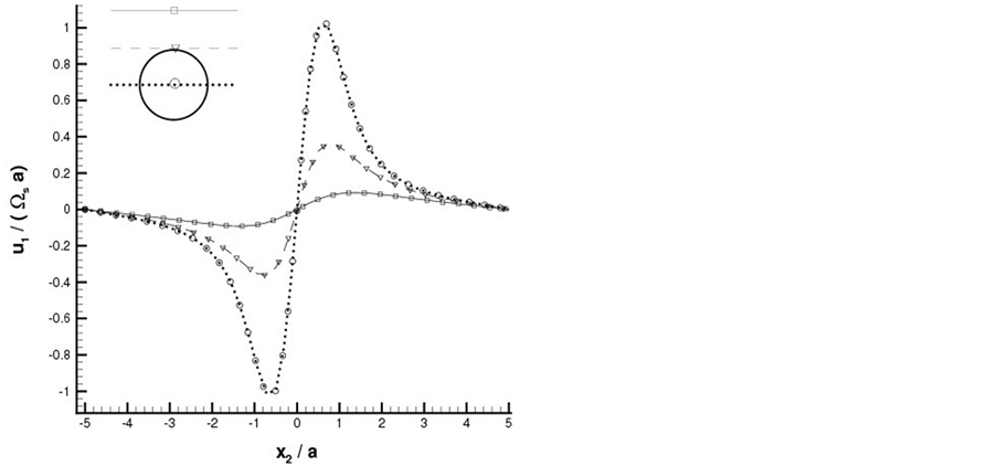

Figure 1. Comparisons of components of fluid velocity profiles across two side walls: (left) u1 velocity in x1; (right) u2 velocity in x2. Symbols are from the author and lines are from Dance [25].
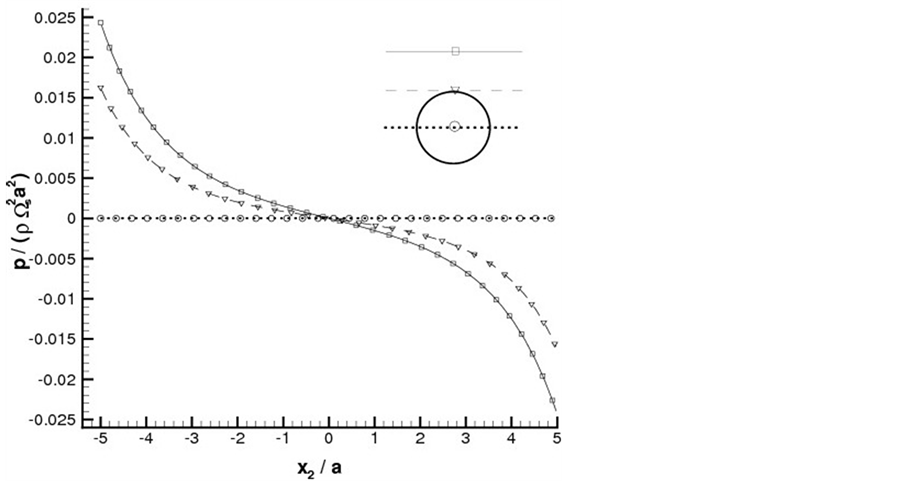
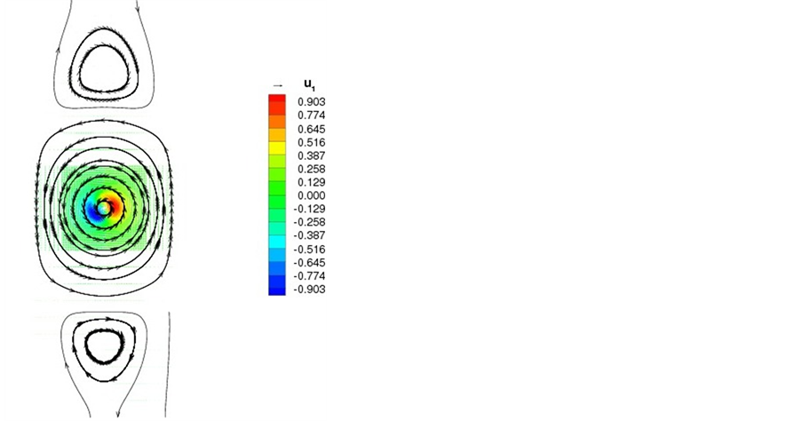
Figure 2. (Left) Comparison of normalized fluid pressure between the author (symbols) and Dance [25] (lines); (Right) Fluid streamlines and contour flood of u1 velocity in x1 in the background.
were specified at boundaries in both  and
and . The dynamic viscosity of the fluid was scaled to be the dimensionless value of
 . The computational volume including the volme inside this sphere was discretized with 256 hexahedral elements and up to 9 quadrature points, i.e., 8th order expansion, were used to ensure enough resolution. To drive the flow, a constant torque normal to the
  plane was applied to the particle’s center. This torque, equivalent to a force dipole, was added into the dipole components
  and
and . Exception the fluid friction and gravitational force, no other force was acting on this particle. The governing momentum equation of the fluid can be simplified as:
 . (15)
In an unbounded domain, this torque would generate an angular velocity of value
 . (16)
But due to the presence of these two side walls at , this particle would be slowed down and the actual angular velocity would be slightly less than one. After convergence tests, the dimensionless angular velocity was
  at the 9th order expansion. Conversely, the direction (sign) of this torque was reversed and the constant torque on the particle was changed to
  and
and . After convergence was reached, the dimensionless angular velocity became
  at the 8th order expansion on every one of 256 elements.
Next, a restoring torque, i.e., a pair of restoring force couples ( and
and ), computed from the penalized Equation (13), was added into the dipole term:
  and
and , in order to slow this particle down from rotation. Therefore, the computation restarted from the previouly converged flow field except no restoring torque. The tolerance for ther residual angular velocity was set to be 0.0075, i.e., 0.75% of the value in Equation (16). Similarly, for the case of the torque with a reversed sign, a corresponding restoring torque was computed to bring the rotating fluid inside the particle into almost stationary.
For the first case with the initial constant torque  and
and , after applying the restoring torque of
  and
and , the angular velocity reduced from
  to
to  which is 0.625% relative to the initial value of
 . For the computed restoring torque, the relative error is 0.875%. If the tolerance for ther residual angular velocity was set to be even smaller, then it is possible to obtain even better results.
For the second case with the initial constant torque  and
and , after applying the restoring torque of
  and
and , the angular velocity reduced from
  to
to . By reversing the torque, the angular velocity data are perfectly reversed. This case verified the penalty algorithm.
Figure 3 (left) demonstrates the angular velocity of this particle versus the dimensionless time. At time is 2, due to the initial constant torque, the angular velocity already reaches 0.9702. Then at time is 10.55, it becomes 0.9898. Starting at time which was 10.55, the restoring started to overcome the initial torque and to slow the spinning of this particle. At time is 11.0, the angular velocity was already reduced to −0.1532; finally at time is 15.5, it was down to 0.0619. This illustrated that the restoring torque works very well and quickly. Figure 3 (right) shows the evolution of the restoring torque. It seems that the angular velocity is very responsive, at the beginning state, to the restoring torque which was added by the penalized differential Equation (13). As the angular velocity gets significantly smaller towards zero, the restoring torque starts to change very little.
Because angular velocity is actually just half of the vorticity of the fluid, vorticity field is plotted to show the details of the flow field. Figure 4 (top) presents the vorticity component of the fluid velocity before adding the restoring torque. In the center of this figure is the volume nominally inside the particle. The advance of VIP is to avoid fully resolving the boundary near the surface of the particle in order to reduce the computational intensity. Therefore, the fluid is actually filled in the particle and tailored force field was computed to simulate the effect of the presence of particle. Because of the nature of added force field, the fluid inside the particle does not perform solid rotational motion, instead, in the figure, the value of the angular velocity is larger at the interior and gradually smaller near the spherical surface. Figure 4 (bottom) is the vorticity field after the restoring torque was fully established. From the ratio of the magnitude of the vorticity, which is essentially the ratio of the angular velocity, the angular velocity was reduced to less than 1% of that without the restoring torque. If using the same scales in the bottom plot, then the fluid is basically without rotation and almost stationary. These plots indicate that the restoring torque and other components of the force dipole can significantly change the flow field
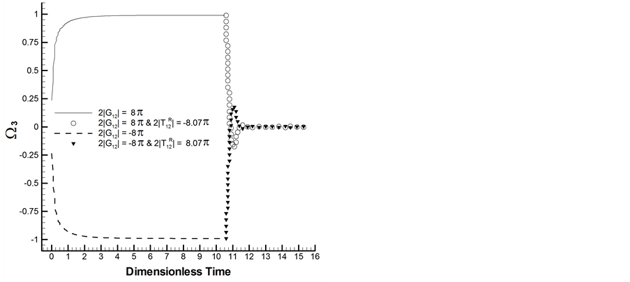
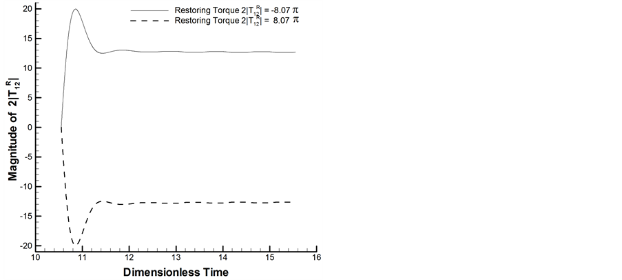
Figure 3. (Left) Evolution of the particle angular velocity before and after restoring torque was added for both positive and negative initial torque; (Right) Evolution of the restoring torque.
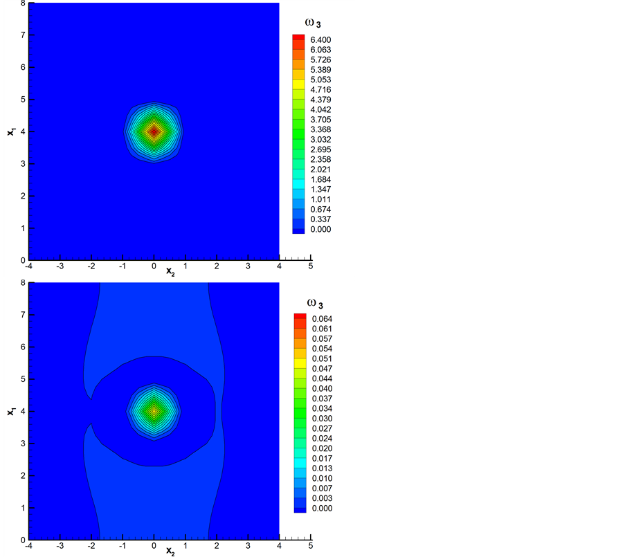
Figure 4. Vorticity contours for flow field before (top) and after (bottom) restoring torque was added.
And the computed force field was successful in modifying the spin of the fluid.
5. Conclusion
The virtual identity particle model was used to model interactions between a rotating particle and the ambient fluid without the demand of curvature-fitted grids/elements near the particle’s surface. Penalized differential equations implemented in the dipole iteration scheme were used to compute the restoring torque to zero out the motion inside the particle. The whole algorithm was implemented with the modal spectral element method which had the reputation for high accuracy and resolvability due to its hierarchically orthogonal bases. Results have been compared with peer’s to validate the algorithm and discussions are made to analyze the intrinsic physics and phenomenon.
Acknowledgements
This work was partially supported by National Science Foundation (Grants DMS-1115546, DMS-1318988, and OIA-1541079). The computational resources were provided by XSEDE (which is supported by National Science Foundation Grant ACI-1053575), Louisiana Optical Network Initiative, and High Performance Computing at Louisiana State University.
Cite this paper
Don Liu,Ning Zhang, (2016) Spectral Element Simulation of Rotating Particle in Viscous Flow. Journal of Applied Mathematics and Physics,04,1260-1268. doi: 10.4236/jamp.2016.47132
References
- 1. Mandø, M., Yin, C., Sørensen, H. and Rosendahl, L. (2007) On the Modeling of Motion of Non-Spherical Particles in Two-Phase Flow. 6th International Conference on Multiphase Flow, ICMF 2007, S2_Mon_D_10, Leipzig, 9-13 July 2007.
- 2. Glowinski, R., Pan, T.W., Hesla, T.I. and Joseph, D.D. (1999) A Distributed Lagrangian Multiplier Fictitious Domain Method for Particulate Flow. International Journal of Multiphase Flow, 25, 775-794. http://dx.doi.org/10.1016/S0301-9322(98)00048-2
- 3. Joseph, D.D. and Ocando, D. (2002) Slip Velocity and Lift. Journal of Fluid Mechanics, 454, 263-286. http://dx.doi.org/10.1017/S0022112001007145
- 4. Johnson, A. and Tezduyar, T.E. (1997) 3D Simulation of Fluid-Particle Interactions with the Number of Particles Reaching 100. Computer Methods in Applied Mechanics and Engineering, 145, 301-321. http://dx.doi.org/10.1016/S0045-7825(96)01223-6
- 5. Maxey, M.R., Patel, B.K., Chang, E.J. and Wang, L.-P. (1997) Simulations of Dispersed Turbulent Multiphase Flow. Fluid Dynamics Research, 20, 143-156. http://dx.doi.org/10.1016/S0169-5983(96)00042-1
- 6. Hu, H., Patankar, N. and Zhu, M. (2001) Direct Numerical Simulations of Fluid-Solid Systems Using The Arbitrary Lagrangian-Eulerian Technique. Journal of Computational Physics, 169, 427-462. http://dx.doi.org/10.1006/jcph.2000.6592
- 7. Liu, D., Maxey, M.R. and Karniadakis, G.E. (2002) A Fast Method For Particulate Microflows. Journal of Microelectromechanical Systems, 11, 691-702. http://dx.doi.org/10.1109/JMEMS.2002.805209
- 8. Markauskas, D., (2006) Discrete Element Modeling of Complex Axisymmetric Particle Flow. Mechanika, 6, 32-38.
- 9. Amsden, A.A. and Hirt, C.W. (1973) YAQUI: An Arbitrary Lagrangian-Eulerian Computer Program for Fluid Flows at All Speeds. Report LA-5100, Los Alamos Scientific Laboratory, Los Alamos.
- 10. Hirt, C.W., Amsden, A.A. and Cook, J.L. (1997) An Arbitrary Lagrangian-Eulerian Computing Method for All Flow Speeds. Journal of Computational Physics, 135, 203-216. http://dx.doi.org/10.1006/jcph.1997.5702
- 11. Apte, S., Martin, M. and Patankar, N.A. (2009) A Numerical Method for Fully Resolved Simulation (FRS) of Rigid Particle-Flow Interactions in Complex Flow. Journal of Computational Physics, 228, 2712-2738. http://dx.doi.org/10.1016/j.jcp.2008.11.034
- 12. Bush, J.W.M., Stone, H.A. and Tanzosh, J.P. (1994) Particle Motion in Rotating Viscous Fluids: Historical Survey and Recent Developments. Current Topics in the Physics of Fluids, 1, 337-344.
- 13. Tanzosh, J.P. and Stone, H.A. (1994) Motion of a Rigid Particle in a Rotating Viscous Fluid: An Integral Equation Approach. Journal of Fluid Mechanics, 275, 225-256. http://dx.doi.org/10.1017/S002211209400234X
- 14. Hynes, J.T., Kapral, R. and Weinberg, M. (1977) Particle Rotation and Translation in a Fluid With Spin. Physica A: Statistical Mechanics and Its Applications, 3, 427-452.
- 15. Bluemink, J.J., Lohse, D., Prosperetti, A. and Wijngaarden, V. (2010) Drag and Lift Forces on Particles in a Rotating Flow. Journal of Fluid Mechanics, 643, 1-31. http://dx.doi.org/10.1017/S0022112009991881
- 16. Liu, Q. and Prosperetti, A. (2010) Wall Effects on a Rotating Shere. Journal of Fluid Mechanics, 657, 1-21. http://dx.doi.org/10.1017/S002211201000128X
- 17. Lee, J. and Ladd, A.J.C. (2007) Particle Dynamics and Pattern Formation in a Rotating Suspension. Journal of Fluid Mechanics, 577, 183-209. http://dx.doi.org/10.1017/S002211200700465X
- 18. Liu, D., Keaveny, E., Maxey, M. and Karniadakis, G.E. (2009) Force Coupling Method for Flows with Ellipsoidal Particles. Journal of Computational Physics, 228, 3559-3581. http://dx.doi.org/10.1016/j.jcp.2009.01.020
- 19. Liu, D., Chen, Q. and Wang, Y. (2011) Spectral Element Modeling of Sediment Transport in Shear Flows. Computer Methods in Applied Mechanics and Engineering, 200, 1691-1707. http://dx.doi.org/10.1016/j.cma.2011.01.009
- 20. Liu, D., Zheng, Y.-L. and Chen, Q. (2015) Grain-Resolved Simulation of Micro-Particle Dynamics in Shear and Oscillatory Flows. Computers and Fluids, 108, 129-141. http://dx.doi.org/10.1016/j.compfluid.2014.12.003
- 21. Kim, S. and Karrila, S.J. (1991) Microhydrodynamics: Principles and Selected Applications. Dover Publications, Inc., Mineola, New York.
- 22. Liu, D. (2004) Spectral Element/Force Coupling Method: Application to Colloidal Micro-Devices and Self-Assembled Particles Structures in 3D Domains. Ph.D. Dissertation, Brown University, Providence.
- 23. Warburton, T.C., Sherwin, S.J. and Karniadakis, G.E. (1999) Spectral Basis Functions for 2D Hybrid hp Elements. SIAM Journal on Scientific Computation, 20, 1671-1695. http://dx.doi.org/10.1137/S1064827597315716
- 24. Karniadakis, G.E. and Sherwin, S.J. (2005) Spectral/hp Element Methods for CFD. Oxford University Press, Oxford. http://dx.doi.org/10.1093/acprof:oso/9780198528692.001.0001
- 25. Dance, S. (2002) Particle Sedimentation in Viscous Fluids. Ph.D. Dissertation, Brown University, Providence.
NOTES

*Corresponding author.